The Counties that Counted: Could 2020 Repeat 2016 in the US Electoral College?
←
→
Page content transcription
If your browser does not render page correctly, please read the page content below
The Forum 2020; 17(4): 675–692

John Agnew and Michael Shin*
The Counties that Counted: Could 2020
Repeat 2016 in the US Electoral College?
https://doi.org/10.1515/for-2019-0040

Abstract: We briefly trace the claim that a set of counties across the three states of
Michigan, Pennsylvania, and Wisconsin in large part determined the outcome of
the 2016 presidential election. Rather than the demographic characteristics of the
Census as such it is the meaning that these categories (young/old, Black/White,
male/female, and so on) take on in particular places in which people’s lives are
grounded that drives electoral outcomes. Given that the counties in question were
ones in which Obama had performed well but which Trump won in 2016 and this
shift was put down to his appeal to those “left behind” in the post-2008 economy,
we focus on whether or not this localized appeal can be expected to continue in
2020.

Introduction
We briefly trace the claim that a set of counties across the three states of Michi-
gan, Pennsylvania, and Wisconsin in large part determined the outcome of the
2016 presidential election. Counties provide an appropriate unit of account given
their significance as administrative units for everyday life and in the context of
a geographically driven electoral system such as the Electoral College. Rather
than the demographic characteristics of the Census as such it is the meaning that
these categories (young/old, Black/White, male/female, and so on) take on in
particular places in which people’s lives are grounded that drives electoral out-
comes. Given that the counties in question were ones in which Obama had per-
formed well but which Trump won in 2016 and this shift was put down to his
appeal to those “left behind” in the post-2008 economy, we focus on whether
or not this localized appeal can be expected to continue in 2020. In particular,
Trump’s performance as president, specifically his use of tariffs in the trade dis-
putes with China and the EU, could be having negative effects in these counties
(and beyond). Of course, much of Trump’s appeal is seen as resting in the status
anxieties of older White voters rather than with respect to this or that economic

*Corresponding author: Michael Shin, (UCLA), Geography, UCLA, Los Angeles CA 90095, USA,
e-mail: shinm@geog.ucla.edu
John Agnew: Geography, UCLA, Los Angeles CA 90095, USA

                                          Brought to you by | Cornell University Library
                                                                         Authenticated
                                                     Download Date | 3/20/20 6:12 PM
676 John Agnew and Michael Shin
issue. Notwithstanding the truth to any of these claims, Trump could still win the
three states even if he loses these counties, by building up bigger majorities in
other counties, but these counties can still be regarded as bellwethers for Trump’s
prospects given the narrow path to re-election that he probably faces.
The 2016 Counties that Counted
One of the major surprises of the 2016 US presidential election was not only that
Donald Trump won but how he won. The voters who determined the outcome
in the Electoral College could all be seated in the University of Michigan foot-
ball stadium. They came from a set of counties across the three states of Michi-
gan, Pennsylvania and Wisconsin which now seem to be the last parts of the US
where voters can switch between presidential candidates of the two main parties
between elections at a time when so many voters appear entrenched in polarized
partisan worlds. Yet, as is known from national polling, the majority of voters
everywhere are not as polarized as the loud voices of politicians and activists in
designating everyone as either a Republican or a Democrat make them appear. It
is just that these potential switchers are frequently swamped in places where the
menu of political choice and the number of partisans leans towards somewhat
fixed outcomes thus leading to the frequently noted, if exaggerated, “red fight-
ing blue” account of homogeneous sectional and state-level political preferences
(e.g. Hopkins 2017).
As a result, it is the places where significant numbers of voters switch politi-
cal preferences across elections that can swing electoral outcomes one way or the
other. They have become increasingly crucial in determining the overall outcome
of US presidential elections. One temptation might be to see these as places with
concentrations of “indifferent” or loosely affiliated voters who switch with ease.
But why there should be so many in small town/rural counties in the states in
question is more mysterious. Implicit attitudes tapped into by Donald Trump but
not previously manifested in political leanings might be more on target (e.g. Ryan
2017). The bombastic and demagogic rhetoric of Trump may indeed have found
resonance precisely with those tired of the pluralism and political correctness
of mainstream US politics looking to blame the problems in their lives on inten-
tional plots against them by shady foes rather than in situational accounts of
forces beyond anyone’s control (e.g. Busby et al. 2019). Rather like Putin in Russia
(Medvedev 2019), Trump has a pick-and-mix ideology with himself at its core and
appeal to nostalgia and resentment of a shifting set of enemies as moments of
mobilization for his fearful “base.” Identifying scapegoats and decrying experts
Brought to you by | Cornell University Library
Authenticated
Download Date | 3/20/20 6:12 PMThe Counties that Counted: Could 2020 Repeat 2016 677
who have failed to address the crises in which many people find themselves
enmeshed prove crucial (e.g. Moffitt 2015; Caramani 2017). Perhaps Trump just
admires the modus operandi of Putin rather than actively colluded with him
during the 2016 election campaign?
The percentage of all counties flipping between parties at subsequent elec-
tions has never been very high over the period 1952–2016, so the counties that do
flip can take on a real significance when elections are tight and a limited number
of states are crucial in the final tally of electoral votes (Sances 2019). From 2004
down through 2016 a set of counties across the upper-Midwest of the US consist-
ently exhibited this quality with others in northern New England and scattered
counties elsewhere waxing and waning in similar volatility. Most of the country
remained locked into consistent local majorities for one or the other party without
much of a shift whatsoever. In 2016 the pattern of consistently volatile counties
finally had a nationwide impact through the mechanism of the Electoral College.
Could this repeat in 2020? Given the overall lack of equivalent historical volatil-
ity in other parts of the country, such as Florida, Arizona, Colorado, and New
Mexico, the upper-Midwest states of Michigan and Wisconsin plus some counties
in Pennsylvania may prove crucial once more whatever the relative disposition of
total votes between parties at the national level. One indicator of this trend that
favors Republican candidates is that from 2013 to 2017 across the most competi-
tive congressional districts nationwide, 8 of 25 of the seats trending Republican
were in Michigan, Pennsylvania, and Wisconsin whereas none of the 25 seats
trending Democrat were in those states (Wasserman and Flinn 2017).
A key element in the outcome of the 2016 presidential election were those
voters largely in the Midwest and Pennsylvania who had backed President
Obama in 2008 (and 2012) but then reversed course to support Donald Trump in
2016. Nationally about 9 percent of Obama voters went for Trump in 2016, about
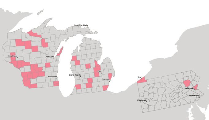
5 percent of the total electorate (Sides et al. 2018). According to Ballotpedia (2017),
206 counties nationwide voted for Trump in 2016 that had voted for Obama in
2008 and 2012. The 206 counties were spread over 34 states. It was where their
numbers were concentrated in key states, however, that was crucial. Michigan
had 12 “pivot” counties, Pennsylvania had 3, and Wisconsin had 23 (Figure 1).
This is where the voters who allowed Trump to eke out his victory in the Elec-
toral College were located as he was massively losing the nationwide popular
vote to Hillary Clinton. Trump won the three states of Michigan, Pennsylvania,
and Wisconsin by net 77,744 votes, mostly concentrated in a number of largely
rural and exurban counties in the three states. These voters seem to be mainly
White working-class voters who never obtained college degrees. Like their peers
across the country, having supported Obama’s campaigns, they turned away from
Hillary Clinton and voted for Trump. If the flipped counties in crucial states had
Brought to you by | Cornell University Library
Authenticated
Download Date | 3/20/20 6:12 PM678 John Agnew and Michael Shin
Figure 1: The Big Three States Showing the Counties that Flipped from Obama (2008 and 2012)
to Trump (2016).
not flipped in 2016, Clinton would have won the Electoral College by 3 votes and
the lowest-educated counties (by average years of education) had voted as they
had in 2012, she would have claimed the Electoral College by around 30 votes
(Sances 2019).
Much speculation and some hard survey data suggest that this was due to
both a sense that Washington during the Obama years had failed to deliver on the
economic front for the vote flippers and their communities and also in reaction to
the increasingly rabid politics of race and policing that had erupted in the second
of Obama’s terms of office (Agnew and Shin 2019, p. 77–81). The relentless federal
focus of the Democratic Party and its relative neglect of state and local politics
probably also fed the sense of neglect (Winter 2019). Trump also was not the
typical Republican candidate; his positions on trade and immigration as well as
his hostility to the “caste” of traditional politicians and bureaucracy matched the
sort of alienation probed in rural Wisconsin by Katherine Cramer (2016) rather
than conventional Republican verities. Overly broad characterizations swept
the places vital to Trump’s election into oppositions such as rural versus urban,
heartland versus coasts, the left behind versus the getting ahead, and White-
nationalist versus globalist America without careful consideration of how eco-
nomic and cultural anxieties intersect on the ground (e.g. Tharoor 2017; Chokshi
2018; Krugman 2018; Neel 2018). Generalization ran ahead of specification.
It is important to note though that the 2016 vote involved a very hard choice.
Neither candidate was particularly popular across the broader electorate. Thus
Brought to you by | Cornell University Library
Authenticated
Download Date | 3/20/20 6:12 PMThe Counties that Counted: Could 2020 Repeat 2016 679
in making a choice, the vote was as much against one of the candidates as in
favor of the other. In 2020 the flipped voters of 2016 will face a president with a
behavioral and policy record, on the one hand, and, at least potentially, a Demo-
cratic candidate without Hillary Clinton’s negative baggage, on the other. After
4 years of partisan squabbling about Trump’s reliance on Russian interventions
in social media in 2016, his impeachment by the US House, and evidence from the
2018 midterm congressional elections that Trump’s often incoherent policies and
unorthodox behavior are far from popular nationally, the 2020 election may not
be a simple shoo-in. Arguably, in 2016 it was as much voters who failed to vote
for Clinton (or anyone else) in the most urban counties who had previously voted
for Obama than it was Obama flippers to Trump who pushed the swing states
over to Trump (Agnew and Shin 2019, p. 77–81). Yet, in 2020, even if incumbency
may benefit a “prizefighter” like Trump, the “illegitimacy benefit” of having won
first time around without winning the popular vote may well weigh against him
(Mayhew 2019, p. 164).
Why Counties Count
In one respect counties are simply accounting units for aggregating votes. Even
though these units nest into the states that are the entities for accumulating the
votes in US presidential elections and reflect the hierarchical territorialism of
US federalism, they need not be understood apart from the sweeping together
of discrete individual persons who are after all the “votes” that ultimately count
in all elections. To make sense of how they vote, we typically understand these
persons in terms of their demographic characteristics (young/old, Black/White,
well educated/poorly educated, affluent/poor, and so on). Yet, the compositional
characteristics of areas like counties (percent over 65, percent Black, etc.) are also
usually taken to signify features of the persons that reflect their life experiences
and outlooks and thus why they vote the ways they do. Analysts are not always
very clear about the fact that these are as much contextual, in the sense of reflect-
ing everyday lives in different places, as they are compositional, reflecting the
presumed common experiences of being Black or elderly wherever you happen to
live in the US. Hillary Clinton’s campaign in 2016 seemed particularly confused
about this fact. Everyone who had voted for Obama anywhere was assumed to be
on track to support Clinton in 2016.
Demographic indicators by themselves even when reported for what turn out
to be “key” counties in electoral outcomes, like those in the Big Three states in
2016, often show few major differences with averages for their respective states
or the states taken together (Table 1). It is how these characteristics and various
Brought to you by | Cornell University Library
Authenticated
Download Date | 3/20/20 6:12 PM680
Table 1: County-Level Demographic Indicators for the Big Three States.
Obama Obama Clinton Trump Margin Counties White African- No Unemployment Median Over Share of total export-
2008 2012 2016 2016 2016 2016 (n) (non- American college income 65 supported jobs
hispanic) under retaliation
US 53.6 51.9 48.3 46.2 3109 61.2 9.1 66 4.7 $50,955 15.2 6.2
John Agnew and Michael Shin
MI-PA-WI 56.7 53.6 47.4 48.2 0.8 222 79.2 3.4 78.4 4.3 $53,072 16.9 6.8
MI-PA-WI- 56.2 53.3 42.6 52.5 9.9 38 .. 3.4 79.9 3.9 $52,204 16.7 ..
flipped
MI 58.4 54.8 47.3 47.6 0.3 83 76.1 4 79.2 5.1 $49,655 17.5 5.9
MI flipped 55.2 52.3 41.8 53.2 11.4 12 .. 5.9 80.1 4.7 $49,411 16.0 ..
PA 55.2 52.7 47.6 48.8 1.2 67 78.6 4.7 77.9 4.5 $54,338 16.7 5.4
PA flipped 56.8 54.2 43.8 52.5 8.7 3 .. 5.4 74.4 4.8 $55,757 16.0 ..
WI 57.1 53.5 47 47.8 0.8 72 82.8 1.6 77.8 3.3 $55,833 16.3 9
WI flipped 57.6 54.2 43.5 51.2 7.7 23 .. 1.8 80.5 3.3 $53,197 17.2 ..
Download Date | 3/20/20 6:12 PM
Authenticated
Brought to you by | Cornell University LibraryThe Counties that Counted: Could 2020 Repeat 2016 681
historical-contextual factors come together that affects the sorts of choices made
by voters on the ground, so to speak. The counties that counted in 2016, therefore,
are not just ones with more less-educated White people over 65 but places where
social class, status anxieties in a changing world, and recent events experienced
there differently from elsewhere combined to produce distinctive electoral out-
comes. Place effects on voting behavior are an emergent phenomenon not simply
reducible to this or that demographic characteristic.
So, we would argue that the context/composition nexus should be made more
explicit. Indeed, before the advent of national opinion surveys and the presumed
nationalization of national politics through communications media and the pro-
jection of national census categories onto the population at large this was what
much electoral analysis tended to do. The presumption was that the act of voting
took place through the prism of the everyday realities facing people that did not
exclude wider influences from beyond the locality but which saw local paths and
practices relating to types of workplaces, religious beliefs, educational opportuni-
ties, and histories of class and racial prejudice as fundamental to political choices.
These are all placed geographically in complex ways that cannot be reduced
readily to the distribution of census categories over space (e.g. Agnew 1987, 1996).
The county, then, can be regarded as much more than just a unit of aggre-
gation. It is potentially a setting where the socio-economic and cultural pro-
cesses emanating locally and from wider networks and relations come together
to provide many of the experiences and outlooks that in turn lead to different
electoral choices. This is not much of a radical claim. Counties have long been
the primary administrative units across much of the US. They are particularly
important as the providers of public goods and services that are vital to people’s
lives from education, police, and public health to roads, transportation, and fire
protection. As Tocqueville was one of the first to note, the history of US settlement
history privileged certain administrative units such as counties as legitimate
political entities that were vital for the very spirit that informed American poli-
tics as it had evolved from independence until when he was writing in the 1830s.
Local affairs and needs were seen as shaping affiliations higher up the territorial
hierarchy of states and the federal government. Arguably, in the face of globaliza-
tion and the retreat of the federal government from earlier interventionist periods
such as the New Deal of the 1930s and the New Society of the late 1960s, the “local
state” has become even more significant politically in people’s lives (Jonas 2002).
Even with the rise of the Web and social media, most people’s online networks
mirror their offline ones with heavy concentrations in their geographical vicinity
(e.g. Dunbar et al. 2015). Counties count, therefore, as politically defined and rel-
evant contexts rather than simply as units of account for the mere accumulation
of individual voter outcomes in geographically organized elections.
Brought to you by | Cornell University Library
Authenticated
Download Date | 3/20/20 6:12 PM682 John Agnew and Michael Shin
Pathways Through the Electoral College
Before the 2016 election, of six scenarios for a pathway to winning the Electoral
College, only one seemed possible for Donald Trump (AEI 2016; Misra 2016). This
had him probably losing the national popular vote but winning Virginia, New
Hampshire as well as Pennsylvania and Wisconsin and missing Michigan. In fact,
he added Michigan to his tally but lost Virginia and New Hampshire. So, Trump’s
pathway to victory was seriously constrained. Yet he prevailed through the Elec-
toral College even while losing the overall nationwide vote mainly because of the
huge majority Hillary Clinton ran up in California. In other words, the Electoral
College matters. What are the likely scenarios for 2020 with respect to plausible
pathways for Donald Trump or his opponent given various assumptions about
his standing and that of possible adversaries? In the subsequent section we then
consider the various factors such as local economic conditions and patterns of
support across the critical counties in the three crucial states in 2016 for a p
ossible
repeat of the 2016 outcome in 2020.
We briefly consider three ways of construing pathways that could lead to the
magic number of 270 Electoral College votes in 2020. Teixeira and Halpin (2019)
provide the first method. This follows the demographic approach pioneered in
AEI 2016. For Trump to win the national popular vote in 2020 he would need to
significantly raise his support among his strongest demographic group: White
non-college voters. If the increase were of the order of 10 percent, Trump would
win the national vote by 1 percent. Increasing support among other demograph-
ics (Blacks, college-educated Whites, etc.) by even 10–15 percent over 2016 would
not lead to a win in the popular vote. None of this matters, of course, on the
ground. The crucial question is where Trump’s support is located relative to his
competitors within the Electoral College.
Under the scenario where turnout and voter decisions by demographic stay
the same as in 2016, and only the overall demography of the electorate in a state
changes (fewer elderly Whites, etc.), Trump would lose Michigan, Pennsylva-
nia and Wisconsin and thus suffer a loss in the Electoral College by a margin
of 279–259 votes. If Black turnout in 2020 follows 2012 rather than 2016, North
Carolina could be added to the list of Trump’s losses. If non-Whites on the whole
swing to the Democratic candidate by 15 points, Florida and Arizona would also
flip from Trump. If college-educated Whites alone were to swing to the Democrat
by 10 points then Arizona, Florida, and North Carolina would join the Big Three
of Michigan, Pennsylvania, and Wisconsin in flipping from Trump.
The best performance scenarios for Trump in the Electoral College require
significant swings in his direction on the part of various demographics. To win
the Big Three and add Maine, Nevada, and New Hampshire into his column, he
Brought to you by | Cornell University Library
Authenticated
Download Date | 3/20/20 6:12 PMThe Counties that Counted: Could 2020 Repeat 2016 683
would need a net shift of 10 percent of non-college educated voters in his direction
leading to a 329-209 victory in the Electoral College. With an unlikely 15 points
shift in his support over 2016 for all non-White groups, Trump would lose the
popular vote but add New Hampshire and Nevada as well as the Big Three to
his column. Finally, if college-educated voters went Trump’s way by 10 points,
he would be edged out in the popular vote but add Maine, Minnesota, and New
Hampshire to his conquests (323–215).
These scenarios assume a uniform swing in turnout and of voter preferences
in different demographics across all states. This is problematic for a number of
reasons. First of all, trends in turnout and preferences vary widely across the
country for the same election. Second, and crucially, the swing states that occur
in all of the above scenarios are ones where all candidates will concentrate their
resources during the 2020 campaign thus affecting the final outcome quite pro-
foundly. At the same time that Trump needs to keep the Big Three in his column,
he must worry that some of the other mentioned states, such as Arizona, Florida,
and North Carolina, could potentially knock him out of contention even if he
retains all of the other states he won in 2016. Trump’s approval ratings by state
and the results of the 2018 Congressional Midterm election will provide his oppo-
sition with a roadmap for exploiting his weaknesses across the Electoral College.
The second method directly uses the results of the 2018 Congressional elec-
tion to map a probability scenario for 2020 (Silver 2018). The scaling up from con-
gressional contests in one election to the presidential ballot 2 years in the future
is obviously fraught. But it does give a more explicitly political picture than the
reliance on demographic groupings tends to do. In aggregate, the 2018 map looks
much more like that of 2012 than that of 2016, suggesting that Trump faces some-
thing of an uphill task if he is to win in 2020. In 2018 Democrats performed par-
ticularly well in Michigan, Pennsylvania, and Wisconsin. The map that emerges
from treating the accumulated congressional votes by state as equivalent to presi-
dential ones looks very much like that of 2012 when Obama defeated Romney.
Interestingly, while Democrats did well overall and in must-win states for them
in 2020, they also performed remarkably well in some states including Arizona,
Iowa, North Carolina, and Texas, where their prospects in 2020 are probably
more questionable. At the same time, states that at one time were seen as bell-
wethers for subsequent presidential elections, such as Missouri and Ohio, defied
the national “trend.” They are now probably not worth the effort to Democratic
presidential candidates in the Trump era.
Even if the 2018 vote is “adjusted” to make it more reflective of the typical
balance in recent years between the parties nationwide, by subtracting 6 percent
from the Democrats’ 2018 margin in every state, Democrats still have an overall
advantage. In this scenario the Big Three once more emerge into prominence. To
Brought to you by | Cornell University Library
Authenticated
Download Date | 3/20/20 6:12 PM684 John Agnew and Michael Shin
win, a Democrat needs these three, what Silver (2018) terms the “Northern Path,”
because, as long as they hold all other states from 2016, they do not need to add
anywhere else. Florida would not be enough as a substitute. They would need
a “Sunbelt Strategy” adding Florida to at least one of Arizona, Georgia, North
Carolina, or Texas as a substitute for the northern route. Crucial to the outcome
is whether the Democratic candidate falls between the two stools provided by the
two pathways. If the southern strategy still does not look “ripe” enough yet demo-
graphically for 2020, the Northern path will therefore be even more central to the
result. As Silver (2018) concludes: “If Trump has lost the benefit of the doubt from
voters in Pennsylvania, Wisconsin and Michigan, he may not have so much of an
Electoral College advantage in 2020.”
Finally, the Big Three and a couple of adjacent states, Iowa and Ohio, can be
considered in light of the overwhelming propensity for Trump to appeal to a spe-
cific demographic/cultural clientele of non-college educated Whites who overlap
with such categories as so-called evangelical voters and those Whites anxious
about their status in an increasingly ethnically and racially diverse country.
During his term of office he has focused on this “base” rather than trying to extend
his constituency very much into other parts of the national population. So, in 2020
this grouping will be even more crucial to his success. As Michael Sances (2019)
shows, since the 1970s educational attainment has become an increasingly power-
ful predictor of US political polarization everywhere. He also demonstrates that
the shift in the vote of the less educated towards Trump in the particular Midwest-
ern states and Pennsylvania was central to the outcome in 2016. Had the coun-
ties in the bottom ten percent of the education distribution stuck with their 2012
preferences, Clinton would have tied with Trump in the Electoral College. If the
bottom 20 percent had done so she would have won. This group of counties was
crucial. They will be again in 2020. And this is so not just because of a singular
demographic trait but also because of a history of electoral volatility combined
with a recent cultural-economic history that is very open to Trump’s messaging.
All three approaches suggest unequivocally that Trump and whomever he
faces in 2020 have relatively narrow pathways to victory. As in 2016, it will likely
be Michigan, Pennsylvania, and Wisconsin that will provide the margin of victory
either way. In all likelihood it will be the counties Sances (2019) identifies within
the three states that will once more loom large on election-day 2020.
2020: 2016 Redux?
So, 2020 may well come down to a scenario remarkably like that of 2016. The
critical question is: what now works for Trump and against him in the crucial
Brought to you by | Cornell University Library
Authenticated
Download Date | 3/20/20 6:12 PMThe Counties that Counted: Could 2020 Repeat 2016 685
counties/states? We examine this question from three viewpoints. The first
relates to Trump’s 2016 explicit appeal to reversing the conventional Republican
positions on trade and industrial policy to emphasize the “disaster” of free trade,
as he saw it, for US workers, particularly those in areas of decline in manufactur-
ing employment. This has led, among other things, to imposing tariffs on imports
from China and other countries, that have then been met with countervailing
ones, targeted expressly at places supportive of Trump in 2016, including agricul-
tural as well as manufactured products. Trump’s positions on trade and manufac-
turing employment appealed directly to groups historically more inclined to vote
Democratic. It also helped him to glue together his overall “base” by opposing his
“nationalism” to the “globalism” that had supposedly caused the depredations
visited on the so-called left-behind in declining industrial areas (Jacobson 2017).
National polling in late 2019 suggests that Trump’s efforts have led to a sig-
nificant increase in support for more open trade rather than the tit-for-tat tariff
policy on which he has embarked. But 2016 Trump voters may in fact see his
efforts more as an effort to “level the playing field” and as temporary measures
rather than seeing him as fundamentally anti-trade (Russonello 2019). Thus
Trump’s trade “war” may still pay off for him in the crucial counties. The national
economy has certainly held up extremely well in the face of the phase of the busi-
ness cycle (in slow expansion since 2012/2013) and in the face of Trump’s trade
measures. So, this is a background condition to the specific effects on the ground
in the localities in question. Yet, through much of 2019 the states of Michigan and
Pennsylvania had decreases in employment particularly in manufacturing and
Wisconsin had only a modest increase in overall employment when many parts
of the country were experiencing net employment growth well above the national
mean (Economist 2019).
In 2016 Trump certainly benefited from his rhetorical flourish about negative
trade impacts and decline in manufacturing employment. Even though much of
the latter can be ascribed to automation more than to the globalization of produc-
tion. Trump’s support grew disproportionately compared to that of Romney in
2012 in places with major declines in manufacturing employment. China was a
more compelling villain than technological change. The impact of the financial
crisis that began in 2007 is also part of this story. Incomes were hit everywhere
but most of all in certain types of place with vulnerable and marginal industries.
The pattern was non-random (e.g. Reeves and Gimpel 2012). The crisis lingered in
its impact in places where industrial decay and hardship had been under way for
years. Much of this was concentrated indeed in less populated, older, Whiter, and
less educated counties in states such as Michigan, Pennsylvania, and Wisconsin
(Noland 2020). Since 2016 these areas have not seen much improvement in their
employment conditions. Since Trump’s arrival in office, Michigan, Pennsylvania,
Brought to you by | Cornell University Library
Authenticated
Download Date | 3/20/20 6:12 PM686 John Agnew and Michael Shin
and Wisconsin in particular have had very low growth in jobs and their manufac-
turing sectors show few if any signs of revival (Casselman and Russell 2019). Of
course, this could be put down to the limited timeframe for national policies to
trickle down to local communities without the advantages in terms of localization
and urbanization economies now largely associated with the largest cities. The
tariff impacts can be used as a surrogate for the overall situation the counties find
themselves in as their previously favored candidate returns to ask for their votes.
We therefore now focus centrally on the geographical impact of tariff meas-
ures in the crucial counties in 2016 and presumably in 2020. After 50 years of
leading efforts to lower barriers to international trade, in 2018 the US govern-
ment enacted several waves of tariffs on specific countries and products. Import
tariffs increased from 2.6 percent to 16.6 percent on 12,043 products covering
about 12.7 percent of annual US imports. In reaction, the affected countries,
mainly China, Mexico, Canada, and the European Union, imposed retaliatory
tariffs on US exports. These measures raised tariffs from 7.3 to 20.4 percent on
8073 products covering 8.2 percent of annual US exports. The county-level expo-
sure to tariff increases was extremely uneven across the country through April
2019 (Fajgelbaum et al. 2019). The largest impact on import declines due to tariff
increases was in the Great Lakes region, southern New England, the Carolinas,
and scattered counties in the West. The major impact of the countervailing tariffs
on US exports was across the Great Plains and the West Coast, and in Texas and
the Mississippi Valley. Regional and local economies specializing in agriculture
and metals have been particularly hit by the countervailing tariffs. Though met-
ropolitan areas have been affected as well, typically the share of exports hit is
much larger percentage-wise in rural areas and small towns. Suggesting at least a
degree of targeting of products by foreign governments, counties won by Trump
in 2016 seem to have been much more exposed to the countervailing duties than
counties that were won by Clinton (Parilla and Bouchet 2018; Fajgelbaum et al.
2019). Even though the tariff war between the US and its partners in NAFTA has
abated, that with China and the EU continues even if in the former case an initial
agreement seems very likely if very incomplete (Bradsher 2019).
Not simply because of the enhanced probability that the flipped counties
of 2016 have faced the negative impact of the tariff wars, it seems that they are
especially vulnerable to such shocks because of the overall vulnerability of their
economies. Examining all of the “pivot counties” nationwide, including those
in the Big Three states, can provide a clue as to the confluence between shocks
such as the tariff increases and ongoing trends in county-level economies. Conse-
quently, it looks very much as if these counties have not only not turned around
since Trump’s election but that they are in fact mired in continuing economic
and demographic stasis (Fikri et al. 2019). Indeed, basic trends are little changed
Brought to you by | Cornell University Library
Authenticated
Download Date | 3/20/20 6:12 PMThe Counties that Counted: Could 2020 Repeat 2016 687
in these counties since 2012 except that in terms of job growth the gap between
these counties and ones that did not flip grew larger between 2016 and 2018. The
same thing went for the growth of business establishments over the same period.
As Fikri et al. (2019) say, if voters truly believe in the powers of a given Presi-
dent to enact economic miracles over a short time, “their hopes have so far been
unfulfilled.”
A second viewpoint moves from the aggregate position relating to the impacts
of tariffs in the counties to considering how much this might matter to the overall
political atmosphere in these places. In other words, we are interested in whether
or not there have been shifts in views of Trump as a net result of the tariff and other
economic measures (tax cuts favoring business, etc.) across affected areas. The
evidence is necessarily very fragmentary but nevertheless suggestive of what can
be seen so far. Historically, states such as Michigan, Pennsylvania, and Wisconsin
have been strongly disputed between the two parties. To win, a presidential candi-
date must take the swing counties in the swing states. Critical to the verdict is how
much the shocks to local communities translate into shifts in turnouts and indi-
vidual votes (e.g. Kiewiet and Lewis-Beck 2011). The community/county define
the settings in which the translation occurs, not “national” economic conditions
per se (although that may have ideological impacts: “He’s doing the right thing
but it just hasn’t worked out around here yet” e.g. Politi 2019) Even if someone is
not immediately on the end of job loss or the fading of employment prospects, the
sight of abandoned factories, declining real estate values, rising drug abuse, and
so on fuel anxiety and anger across the local populace (e.g. Reeves and Gimpel
2012; Ansolabehere et al. 2014). This is also the case in predominantly agricul-
tural counties where most of the population is not directly employed in farming
any more but the economic health of the farming sector drives the prospects for
all of the other businesses and people in the vicinity.
It is now something of conventional wisdom that economic changes are
mediated in their effects on voting in complex ways, particularly in relation to
anxieties about social status and worries about the future beyond whether or not
jobs are growing or trading with foreign countries is “unfair.” Indeed, it may well
be Trump’s populist rhetoric, notwithstanding its negative material impacts, that
continues to attract voters. The increasingly polarized electorates, including now
those in the Obama-Obama-Trump counties in question, may be less swayed than
in the past by how well the economy is or is not doing (Ip 2019). Issues of race,
immigration, and gender dominated the 2016 campaign more than economic
issues per se. National survey evidence suggests strongly that the voting gap
by education-level for Trump cannot be adequately explained solely in terms of
economic difficulties. Attitudes on race and gender strongly channeled the direc-
tion of votes in 2016 (Schaffner et al. 2018). Given that it was non-college Whites
Brought to you by | Cornell University Library
Authenticated
Download Date | 3/20/20 6:12 PM688 John Agnew and Michael Shin
whose flipping largely led to the outcomes in the counties of the Big Thee states
in 2016 it seems that this relationship holds for them too. Whether this was an
aberration of a year in which the first woman presidential candidate was running
against someone who made unrestrained use of racist and misogynistic tropes
and gestures in the aftermath of a two-term African-American President is impos-
sible to say. What it does suggest is that we cannot simply assume a straightfor-
ward causal arrow going from recent economic trends to voting outputs. This is
particularly the case, as was noted earlier (see, e.g. Ryan 2017; Busby et al. 2019),
for a set of places in which a history of relatively weak partisan affiliations in a
substantial section of the local population has led to swings in voting behavior
that led to the exposure of implicit attitudes with the emergence of a candidate
like Donald Trump’s whose appeal is not really to either a conventional Republi-
can constituency or to the more urban-liberal ethos of today’s Democratic Party
but to a populist base alienated from all politics-as-usual.
From the third viewpoint, we are interested in how this all adds up to in terms
of the likely prospects for Trump in 2020. With respect to the crucial counties in
the Big Three states, the demography of employment would seem in theory to
favor a Democrat over Trump; workers in service employment now far outnumber
those in manufacturing and transportation. But the prospect for manufacturing
tends to color the vibrancy of work in these other sectors: it has bigger multi-
plier effects across local economies. There are relatively few foreign immigrants
in most of these counties. But absence does not always make the heart grow
fonder. The counties are overwhelmingly White relative to the national average.
They also have relatively high shares of the non-college educated, as noted previ-
ously. They also have relatively older populations (Fikri et al. 2019; McGraw 2019).
Yet, 2019 survey evidence from the Big Three states suggests that Trump cannot
be written off for 2020; far from it. Trump’s approval rating even while low and
largely stagnant nationally since coming into office has risen in the crucial coun-
ties (e.g. Saul and Peters 2019; Zitner and Chinni 2019). This is despite the lack of
much by anything of major economic improvement and in the face of being in the
trenches of the tariff wars. The signs of a drawdown in the tariff war with China
in late 2019 and the passage of the updated NAFTA trade deal with Canada and
Mexico may improve Trump’s prospects (Rappeport et al. 2019). Trump has other
things going for him too, particularly his demagoguery on race and immigration
(Guo 2016). Trump overcame weak approval and favorability ratings in 2016. In
2020 he can point to the “partisan” impeachment effort by Democrats in 2019,
whatever the evidence of criminality he was involved in, to once more portray
himself as an outsider, sowing chaos in Washington and around the world on
behalf of “the people.” Whether Democrats can mobilize around the impeach-
ment to limit Trump to a single term is a very open question (Balz 2019b).
Brought to you by | Cornell University Library
Authenticated
Download Date | 3/20/20 6:12 PMThe Counties that Counted: Could 2020 Repeat 2016 689
Of course, his prospects in 2020 depend on what sort of candidate he faces
this time around. Last time around he had one who shared his low favorability
rating. Since coming into office Trump has done nothing to expand his base. “The
wild card,” as the journalist Dan Balz (2019a) makes the point: “is the identity of
the Democratic nominee and how that shapes the general election debate. Will
that nominee be running on a platform that moderate voters see as too far left?
Will that nominee be able to energize the party’s woke base and still appeal to
White working-class voters.” This perspective also engages the relative turnout
question. Older, more conservative American voters have a greater propensity to
vote than other demographic groupings. This is undoubtedly in Trump’s favor
(Leonhardt 2016; Jacobs 2019). Even if in 2016 the overall role of relative turnout
on each side could be exaggerated (e.g. Cohn 2017), its importance in the Big
Three states, particularly in urban counties where Obama had reaped high rates
of voting by African Americans and Clinton did not, was significant in the story of
the outcome in the three states. It could be again. In obvious counterpoint, in the
crucial counties in those very states what matters most of all, if recent research on
the topic is to be believed, is that in places with a history of swing voters a party
that nominates a more “extreme” candidate, rather than mobilizing the hitherto
uninvolved as “mobilization theory” would predict, tends to bring out voters on
the other side in increased numbers (Hall and Thompson 2018). Trump could very
well trump himself in the right places from 2016 with the right candidate on the
other side. 2020 will test this thesis on the ground.
Conclusion
In brief compass, we have described the counties in the US that counted most in
the outcome of the 2016 presidential election because of the nature of the Elec-
toral College as a mediating mechanism. Using counties, however, is not simply
because they are units of account for votes but also because they are contexts in
which people are exposed to differing experiences and influences that affect their
vote choices. Of course, these places are not isolated but they still provide domi-
nant settings in which everyday lives are lived. We then traced the ways in which
the Electoral College in 2020 might follow the pattern established in 2016 with
the Northern Pathway involving the crucial 2016 counties in the Big Three states
as the most likely one again in 2020. Finally, we weighed up the pros and cons
of recent economic impacts, particularly Trump’s tariff wars, on the counties in
question and how the effects might play out in 2020. Our conclusion is that Trump
could very well succeed again. Trump’s electoral appeal is not ultimately based
in economic issues per se. His standing with indifferent swing voters is such that
Brought to you by | Cornell University Library
Authenticated
Download Date | 3/20/20 6:12 PM690 John Agnew and Michael Shin
he just needs enough of them to show up to outnumber the other side. If he cam-
paigns as he did in 2016, by stoking anger and hostility against their “adversar-
ies,” he could do this once more.
References
Agnew, J. 1987. Place and Politics: The Geographical Mediation of State and Society. London:
Allen and Unwin.
Agnew, J. 1996. “Mapping Politics: How Context Counts in Electoral Geography.” Political Geog-
raphy 15 (2): 129–146.
Agnew, J., and M. Shin. 2019. Mapping Populism: Taking Politics to the People. Lanham, MD:
Rowman and Littlefield.
American Enterprise Institute (AEI). 2016. A New Look at How Demographic Shifts in Race, Age,
and Generation Could Affect Future Election Outcomes, (from 2016 to 2032). Washington,
DC: AEI.
Ansolabehere, S., M. Meredith, and E. Snowberg. 2014. “Mecro-Economic Voting: Local Informa-
tion and Micro-Perceptions of the Macro-Economy.” Economics and Politics 26: 380–410.
Ballotpedia. 2017. Pivot Counties: The Counties that Voted Obama-Obama-Trump from 2008-
2016. https://ballotpedia.org/pivot_counties:_the_counties_that_voted_Obama_Obama_
Trump_from_2008-2016.
Balz, D. 2019a. “The 2020 Electoral Map Could Be the Smallest in Years. Here’s Why.” Washing-
ton Post, 31 August.
Balz, D. 2019b. “Will Impeachment Be Forgotten by November 2020? Don’t be So Sure.” Wash-
ington Post, 7 December.
Bradsher, K. 2019. “China’s Hard-liners Win a Round in Trump’s Trade Deal.” New York Times,
14 December.
Busby, E. C., J. R. Gubler, and K. A. Hawkins. 2019. “Framing and Blame Attribution in Populist
Rhetoric.” Journal of Politics 81 (2): 616–630.
Caramani, D. 2017. “Will vs. Reason: The Populist and Technocratic Forms of Political Representa-
tion and their Critique of Party Government.” American Political Science Review 111 (1): 54–67.
Casselman, B., and K. Russell. 2019. “There are Economic Warning Signs for Trump in the Mid-
west.” New York Times, 16 December.
Chokshi, N. 2018. “Trump Voters Driven by Fear of Losing Status, Not Economic Anxiety, Study
Finds.” New York Times, 24 April.
Cohn, N. 2017. “A 2016 Review: Turnout Wasn’t the Driver of Clinton’s Defeat.” New York Times,
28 March.
Cramer, K. J. 2016. The Politics of Resentment: Rural Consciousness in Wisconsin and the Rise of
Scott Walker. Chicago: University of Chicago Press.
Dunbar, R. I. M., V. Arnaboldi, M. Conti, and A. Passarella. 2015. “The Structure of Online Social
Networks Mirrors Those in the Offline World.” Social Networks 43: 39–47.
Economist. 2019. “Parts of America may Already be Facing Recession.” 31 August. https://
www.economist.com/united-states/2019/08/31/parts-of-america-may-already-be-facing-
recession.
Fajgelbaum, P., P. K. Goldberg, P. J. Kennedy, and A. K. Khandelwal. 2019. The Return of
Protectionism. Cambridge, MA: National Bureau of Economic Research.
Brought to you by | Cornell University Library
Authenticated
Download Date | 3/20/20 6:12 PMThe Counties that Counted: Could 2020 Repeat 2016 691
Fikri, K., A. Benzow, and N. Esposito. 2019. The Flipped Counties of 2016 Still Lagging Behind.
Washington, DC: Economic Innovation Group.
Guo, J. 2016. “Yes, the Working Class Whites Really Did Make Trump Win. No, It wasn’t Simply
Economic Anxiety.” Washington Post, 11 November.
Hall, A. B., and D. M. Thompson. 2018. “Who Punishes Extremist Nominees? Candidate Ideol-
ogy and Turning Out the Base in US Elections.” American Political Science Review 112 (3):
509–524.
Hopkins, D. A. 2017. Red Fighting Blue: How Geography and Electoral Rules Polarize American
Politics. Cambridge: Cambridge University Press.
Ip, G. 2019. “‘It’s Not the Economy Anymore, Stupid.” Wall Street Journal, 12 November.
Jacobs, T. 2019. “Trump Supporters are more Likely to Vote than Trump Opponents.” Pacific
Standard, 11 July.
Jacobson, G. C. 2017. “The Triumph of Polarized Partisanship in 2016: Donald Trump’s Improb-
able Victory.” Political Science Quarterly 132: 9–41.
Jonas, A. 2002. “Local Territories of Government: From Ideals to Politics of Place and Scale.” In
American Space/American Place: Geographies of the Contemporary United States, edited
by J. Agnew and J. Smith, 108–149. Edinburgh: Edinburgh University Press.
Kiewiet, D. R., and M. S. Lewis-Beck. 2011. “No Man is an Island: Self-Interest, the Public Inter-
est, and Sociotropic Voting.” Critical Review 23 (3): 303–319.
Krugman, P. 2018. “What’s the Matter with Trumpland?” New York Times, 2 April.
Leonhardt, D. 2016. “The Democrats’ Real Turnout Problem.” New York Times, 17 November.
Mayhew, D. R. 2019. “Incumbency Advantage in U.S. Presidential Elections: the Historical
Record.” In Presidential Selection and Democracy, edited by D. J. Caraley and R. Y. Shapiro.
New York: Academy of Political Science.
McGraw, D. 2019. “How These Seven Counties Could Shape the 2020 Election.” The Bulwark,
March. http://thebulwark.com/how-these-seven-counties-could-shape-the-2020-election.
Medvedev, S. 2019. The Return of the Russian Leviathan. Cambridge, England: Polity.
Misra, T. 2016. “Demography Favors the Democrats.” CityLab, 26 February. https://www.citylab.
com/equity/2016/02/demography-favors-the-democrats/470937/.
Moffitt, B. 2015. “How to Perform a Crisis: A Model for Understanding the Key Role of Crisis in
Contemporary Populism.” Government and Opposition 50 (2): 189–217.
Neel, P. A. 2018. Hinterland: America’s New Landscape of Class and Conflict. London: Reaktion.
Noland, M. 2020. “Protectionism Under Trump: The China Shock, Deplorables, and the First
White President.” Asian Economic Policy Review 15 (1): 31–50.
Parilla, J., and M. Bouchet. 2018. “Which US Communities are Most Affected by Chinese, EU,
and NAFTA Retaliatory Tariffs?” Brookings Report, October.
Politi, J. 2019. “Donald Trump’s Struggle to Revive the US Rust-Belt.” Financial Times,
30 November.
Rappeport, A., A. Swanson, K. Bradsher, and C. Buckley. 2019. “Initial Deal De-escalates Trade
War with China.” New York Times, 14 December.
Reeves, A., and J. G. Gimpel. 2012. “Ecologies of Unease: Geographic Context and National
Economic Evaluations.” Political Behavior 34 (3): 507–534.
Russonello, G. 2019. “Trump is Pushing Protectionism. But Polls Show Americans Embracing
Trade.” New York Times, 6 December.
Ryan, T. J. 2017. “How Do Indifferent Voters Decide? The Political Importance of Implicit Atti-
tudes.” American Journal of Political Science 61 (4): 892–907.
Sances, M. W. 2019. “How Unusual was 2016? Flipping Counties, Flipping Voters, and the
Education-Party Correlation since 1952.” Perspectives in Politics 17 (3): 666–678.
Brought to you by | Cornell University Library
Authenticated
Download Date | 3/20/20 6:12 PM692 John Agnew and Michael Shin
Saul, S., and J. W. Peters. 2019. “In Conservative Michigan, Voters Want to Love Trump, Not
Leave Him.” New York Times, 22 July.
Schaffner, B. F., M. Macwilliams, and T. Nteta. 2018. “Understanding White Polarization in the
2016 Vote for President: The Sobering Role of Racism and Sexism.” Political Science Quar-
terly 133 (1): 9–34.
Sides, J., L. Vavreck, and M. Tesler. 2018. Identity Crisis: The 2016 Presidential Campaign and
the Battle for the Meaning of America. Princeton, NJ: Princeton University Press.
Silver, N. 2018. The 2018 Map Looked a Lot Like 2012 … And that Got Me Thinking about 2020,
Fivethirtyeight.com/features/the-2018-map-looked-a-lot-like-2012-and-that-got-me-think-
ing-about-2020.
Teixeira, R., and J. Halpin. 2019. The Path to 270 in 2020. Washington, DC: Center for American
Progress.
Tharoor, I. 2017. “Trump and the Populists See Themselves at War with Big Cities.” Washington
Post, 20 March.
Wasserman, D., and A. Flinn. 2017. “Introducing the 2017 Cook Political Report Partisan Voter
Index.” The Cook Political Report, April 7.
Winter, M. 2019. All Politics is Local: Why Progressives Must Fight for the States. New York: Bold
Type.
Zitner, A., and D. Chinni. 2019. “Slow Growth Hasn’t Hurt Trump in Key Midwest Counties.” Wall
Street Journal, 13 September.
John Agnew is Distinguished Professor of Geography at UCLA. His research and teaching inte-
rests are in comparative electoral geography, the geopolitics of the world economy, and globa-
lization and sovereignty. His most recent books are (as co-editor) Handbook of the Geographies
of Power (2018) and (as co-author) Mapping Populism: Taking Politics to the People (2019).
Michael Shin is Professor of Geography at UCLA. He specializes in comparative electoral geo-
graphy, GIS, and cartography. His most recent book (as co-author) is Mapping Populism: Taking
Politics to the People (2019).
Brought to you by | Cornell University Library
Authenticated
Download Date | 3/20/20 6:12 PMYou can also read