THE DANGEROUS FICTION OF THE "FISCAL BLACK HOLE" - HOW ARBITRARY TARGETS AND UNCERTAIN FORECASTS ARE DRIVING A RETURN TO AUSTERITY

BRIEFING

THE DANGEROUS FICTION OF THE
“FISCAL BLACK HOLE”
HOW ARBITRARY TARGETS AND UNCERTAIN FORECASTS ARE DRIVING
A RETURN TO AUSTERITY

Rob Calvert Jump and Jo Michell
November 2022

Executive Summary

Media reporting of the economy and choices facing the new Prime Minister and Chancellor
has focused on a supposed ‘black hole’ in the public finances, typically given as being around
£50bn in five years’ time. This has been presented as an urgent priority for government to
fix, and both the Chancellor and Prime Minister have stressed that a return to austerity and
spending cuts is now needed.
Yet this fiscal ‘hole’ is the product of forecasts produced by economic models and the
government’s own fiscal rules. Its size depends on how much we think the economy will
grow, what interest rate the government must pay on its borrowing, and the target for the
size of the government’s debt relative to the size of the whole economy (the ‘debt to GDP
ratio’).
This means that the so-called fiscal ‘hole’ is not an objective statement of economic fact in
the same way that, for example, estimates of current inflation and wage rises are. It is
dangerously misleading to present it as if it was.
Forecasts from economic models are highly uncertain, but this uncertainty is not being
reported properly. The rate of future economic growth, the level of future interest rates, and
the nature of the fiscal target will dramatically alter the size of the so-called fiscal ‘hole’.
Using the Office for Budget Responsibility’s own forecasts, we show that estimates of the
fiscal ‘hole’ are highly sensitive to small changes in future growth rates or interest rates.
Remarkably, using these forecasts, a ‘black hole’ as large as £50bn could be eliminated
simply by reverting to the official measure of public debt used 18 months ago, and
even £14bn of extra spending would not bring it back.
Specifically, the government used to target the public sector net debt including the Bank of
England but changed this to the public sector net debt excluding the Bank of England at the
beginning of this year. This small change has a huge impact on whether the government’s
target is hit – far bigger than any actual policy changes. Including the Bank of England in the
government’s target, for instance, means that the targeted measure of debt would be forecast
to fall by around £64bn in five years’ time – easily more than the so-called ‘black hole’, and
more than the current round of cuts and tax rises being trailed in advance of the Autumn
statement.
Pushing spending cuts to chase a target that is highly uncertain and affected by factors over
which the government has very limited control is bad economic policy, made at high cost
with limited chance of success.
Any fiscal difficulties that the government currently faces have little to do with control of
departmental spending, investment, or taxation. Instead, they are based on arbitrary targets,
and contingent on projected borrowing costs and growth rates which are both subject to
significant levels of uncertainty.

It makes no sense to pre-empt any potential increases in borrowing costs with a
return to austerity. We do not know what the cost of government borrowing will be.
We do not know what nominal GDP will be. We do, however, know all too well what
the cost of austerity would be.
A rational policy response at this point in time would be a cautious, ‘wait and see’ approach.
Spending should not be cut, while taxes on higher earnings and income from wealth could
reasonably be increased to cover any further increases in borrowing costs if they occur. For
an interactive tool to explore these options, see https://arunadvani.com/taxreform.html.

Introduction
In the run up to the November 2022 Autumn Statement there has been sustained discussion
of so-called ‘holes’ in the public finances, and of the spending cuts and tax increases allegedly
needed to fill them. The public is given the impression of an urgent need to prevent an
impending disaster driven by out-of-control public finances.
However, explanation of how the size of these ‘holes’ is calculated is rarely provided, while
justification for their existence usually relies on appeals to reputable organisations such as
the Institute for Fiscal Studies, the Resolution Foundation, or the Office for Budget
Responsibility.
Those following the economic news might reasonably be confused: if September’s ‘mini-
budget’ has been abandoned, why are we not back to square one? If there was no
requirement for Osborne-style austerity before Kwasi Kwarteng’s ill-timed experiment, why
is the media now awash with talk of spending cuts?
Claims about the existence of ‘holes’ in the public finances are based on two elements. First,
some future target or ‘fiscal rule’ is announced, usually by the government. Second, forecasts
or projections of the public finances are produced. The difference between the numbers in
these forecasts and the government’s targets are then calculated.
The difference between forecasts and targets is what is reported to the public as a fiscal
‘hole’. Usually, the impression is given that some specific amount of money needs to be saved,
along with a sense of inevitability about the numbers. What is often missing is any discussion
of whether the targets are meaningful, or whether the predictions are reliable.
In reality, these ‘holes’ are artificial and uncertain. They are artificial because they are based
on arbitrary targets announced by the government. They are uncertain because they rely on
forecasts of key macroeconomic and financial variables several years in the future. These
variables are difficult to predict, and changes in growth rates or interest rates can have a
large effect on how far fiscal variables end up from their targets.
This is why the size of fiscal ‘holes’ reported in the press can appear to vary by tens of billions
of pounds from one week to the next. Various estimates over the last six weeks have put the
figure at £35 billion, £40 billion, or £50 billion. To put these figures into context, this is in the
order of the annual cost of employing one million nurses. Meanwhile, the media are trailing
a figure of £60 billion in spending cuts and tax rises in the August statement.
In this report, we explain how these projections are calculated and provide some illustrative
scenarios for the public finances under a range of plausible assumptions. We show how small
changes in interest rates, growth rates, and changes to the Bank of England’s balance sheet
each have significant effects on forecasts. The difficulty of forecasting these variables feeds
directly into the instability of the claimed ‘holes’ in the public finances.

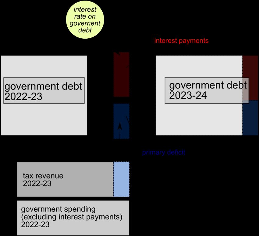
Importantly, variables under direct government control – taxation and spending – have less
impact on whether targets are reached than variables outside direct control. The current
government’s target is a falling debt-to-GDP ratio three to five years in the future, but the
direct effects of changes in spending and taxation are less important in achieving this than
the interest rate on government debt and the growth rate of GDP. And seemingly minor
changes to the type of debt targeted have a huge impact on whether the government’s target
is hit – far bigger than any policy changes.
In an increasingly uncertain world, gilt yields and growth rates cannot be forecast with any
degree of certainty. The costs of austerity, on the other hand, are now well-known. Recent
estimates put the cost of Osborne’s fiscal policies at over 300,000 excess deaths.1 It is widely
accepted that austerity contributed to weak growth, and thus was self-defeating even in
terms of the stated objective of lowering debt-to-GDP ratios.2
We argue that uncertain fiscal projections cannot be used to justify a return to austerity. The
government would be better advised to completely reverse the mini-budget, stick to its
current spending plans, and respond to any increases in borrowing costs – if they materialise
– with taxation on higher earners and the wealthy.

How are projections of the public finances created?
Fiscal projections aim to present plausible, logically coherent stories about how government
borrowing and interest payments might change over time. To generate these projections,
some straightforward accounting is used, as summarised visually in Figure 1.
Given a stock of government debt at the end of a period of time (usually the end of a fiscal
year, which is measured from the start of April to the end of the following March) we want
to know how much the stock of debt will have increased by the end of the next period (e.g.,
the end of the next fiscal year).
One way to visualise the factors that drive increases in debt over each period is to split the
overall increase – the deficit – into two components. The first is the amount spent on interest
payments during the period. This is determined by two things: the interest rate on
government debt, and the size of the debt. The second component is the primary deficit. This
is the difference between government spending (excluding interest payments) and taxation.
The increase in government debt each year is the sum of the primary deficit and interest

1Walsh D, Dundas R, Mc Cartney G, Gibson G, Seaman R., “Bearing the burden of austerity: how do changing
mortality rates in the UK compare between men and women?” Journal of Epidemiology & Community Health,
pre-publication. https://jech.bmj.com/content/jech/early/2022/09/26/jech-2022-219645.full.pdf
2See, for a numerical example, Alfie Stirling, “Austerity is subduing UK economy by more than £3,600 per
household this year”, New Economics Foundation, 21 February 2019.
https://neweconomics.org/2019/02/austerity-is-subduing-uk-economy-by-more-than-3-600-per-
household-this-year

payments (plus certain stock-flow adjustments; we explain the algebra behind figure 1 in
more detail in the appendix).

 Figure 1: The mechanics of an increase in government debt

In order to calculate how the debt stock will change between one period and the next, we
therefore need to know three things: the size of the debt stock, the interest rate on the debt,
and the primary deficit.
For example, if the public debt at the end of last year was £100bn, the interest rate on that
debt is 3%, and the primary deficit over the course of this year is £5bn, then the debt stock
will increase by £8bn over the course of this year (£3bn of interest payments plus the £5bn
primary deficit), resulting in a debt stock at the end of this year of £108bn. If the interest rate
remains at 3%, then interest payments will increase to around £3.25bn next year, because
the debt stock has increased.
Instead of considering debt and interest payments in cash terms, however, it is more useful
to compare these measures to national income (GDP) or tax revenues. This is because GDP
and tax revenues usually increase each year (outside of recessions), meaning that more
income is available to cover interest payments. If GDP grows faster than the debt stock, then
the debt-to-GDP ratio will fall over time. We therefore consider the main variables – debt,
interest payments and the primary deficit – calculated as percentages of GDP.
If we want to know what will happen to the debt, the deficit, and interest payments as
percentages of GDP, we need to know the following: the current debt-to-GDP ratio, the

expected path of the primary deficit-to-GDP ratio, the expected interest rate on government
debt, and the expected growth rate of GDP.
These are the inputs into any fiscal forecasting exercise. They are also, with the exception of
the current debt-to-GDP ratio, unknown. The interest rate on government debt and the rate
of GDP growth, in particular, are very difficult to forecast over a five year horizon with any
degree of certainty.
While we know, therefore, that the public debt will tend to increase relative to GDP when
interest rates increase, when GDP growth slows, or when the public sector borrows more, it
is impossible to produce forecasts of these variables with high degrees of certainty attached.
Nevertheless, reputable organisations continue to produce projections, and these are
reported in the media with little explanation or regard for their uncertainty. Moreover,
media discussion tends to focus on the effects of spending and taxation – despite the fact the
changes in interest rates and growth rates can be just as important – and avoid critical
discussion of the validity of the targets these projections are compared to.
In the following section we present scenarios which illustrate the problems with this
approach.

Illustrative scenarios for the public finances
Changes to the primary deficit
We first consider three scenarios with identical projected GDP growth and interest rates, but
different trajectories for the primary deficit. These are summarised in figure 2, which shows
the primary deficit, interest payments on public debt and public sector net debt, all as a
percentage of GDP, over a five year forecast horizon.
The baseline scenario is essentially the same as the Office of Budget Responsibility’s March
2022 projections, with one percentage point added to the government’s borrowing costs to
take into account recent increases in Bank rate, gilt yields, and inflation (which feeds into
borrowing costs on index-linked gilts). Debt starts falling in this scenario, relative to GDP, by
the 2023-24 fiscal year.
Since then, an energy support package was announced in May, an energy price guarantee
was announced in September, Kwasi Kwarteng announced his mini-budget later in
September, and Jeremy Hunt announced his partial reversal of the mini-budget in October.
The second and third scenarios in figure 2 incorporate Kwasi Kwarteng’s mini-budget and
Hunt’s partial reversal, respectively, with both scenarios incorporating the May energy
support package. Figure A.1 in the appendix provides time paths (and historical information)
for the other variables in the ‘partial mini-budget reversal’ scenario.
The implied additions to public sector borrowing over and above the baseline projection are
displayed in table 1, with every other aspect of the baseline held constant. We explain the
details of how we arrive at the numbers in table 1 in the appendix.

Figure 2: Effects of changes to the primary deficit

Clearly, as illustrated in figure 2, the energy support policies and Kwarteng’s mini-budget
would have added substantially to public sector net debt. But their partial reversal by the
new Chancellor brings the borrowing trajectory to just above the OBR’s March projection
(allowing for increased interest rates) by 2024-25, and the primary deficit is essentially in
balance. The debt-to-GDP ratio stabilises, and then starts to fall, within three years.

 Table 1: additions to public sector borrowing above March 2022 OBR forecast from
 Kwarteng “Growth Plan” and Hunt partial reversal, 2022-27 (£bn)

 Scenario: 2022-23 2023-24 2024-25 2025-26 2026-27
 Growth Plan: 79 58 31 39 45
 of which: May 15 0 0 0 0
 energy support
 of which: Sept. 60 31 0 0 0
 energy support
Partial reversal: 75 8 12 16 19
 of which: May 15 0 0 0 0
 energy support
 of which: Sept. 60 0 0 0 0
 energy support

Figure 3: Effects of changes to borrowing costs

Changes to interest rates and growth rates
While there is some uncertainty associated with the time path of the primary deficit, this is
largely within the Treasury’s control – we know with, for example, that the majority of the
‘mini-budget’ decisions have now been reversed. Any remaining uncertainty is, therefore,
limited.
Instead, the majority of the forecast uncertainty is associated with the future trajectories of
interest rates and growth rates, which are outside the Treasury’s direct control. To illustrate
the first of these sources of uncertainty, in figure 3 we present potential scenarios for
government borrowing costs over and above the scenario for Hunt’s partial reversal of the
mini-budget. As demonstrated in figure 3, the public finances are currently on a knife-edge,
such that their trajectory over the next five years will depend heavily on what happens to
borrowing costs. With government borrowing costs just 2 percentage points higher, the
debt-to-GDP ratio under the Hunt plan evolves in a very similar manner to the debt-to-GDP
ratio under the ‘mini-budget’ scenario in figure 2.
The effects of falling GDP growth rates are similar to those of rising interest rates: any fall in
GDP will tend to increase the debt-to-GDP ratio automatically. This is illustrated in figure 4,
which plots three potential scenarios for nominal GDP growth over and above the scenario
for Hunt’s partial reversal of the mini-budget. A nominal GDP growth rate just 1 percentage
point lower than the OBR’s March 2022 forecast has a similar effect on the debt-to-GDP ratio
as a 2 percentage point increase in borrowing costs, while a higher growth rate leads to a
debt-to-GDP ratio that falls comfortably, as a share of GDP, by the end of the forecast horizon.

Figure 4: Effects of changes in growth rates

Unfortunately, the time-path of nominal GDP is just as difficult to forecast as interest rates in
today’s environment of heightened uncertainty. This is because the relevant measure is
nominal (i.e., cash-terms) GDP. The lengthy recession expected by the Bank of England will
reduce cash-terms GDP, while raised inflation will increase it; the net effect of these two
opposing forces is very difficult to foresee.
It is also important to note that while growth and interest rates are not under the direct
control of the Treasury, these variables are nevertheless affected by decisions over taxation
and spending. It is widely accepted that government spending causes a ‘fiscal multiplier’
effect: increased government spending does not only show up as higher borrowing, but also
as higher GDP. Thus, cuts to government spending will likely lead to lower than previously
expected GDP and thus higher debt-to-GDP ratios. The relevance of these multiplier effects
was highlighted in a recent quote in the Financial Times referring to a £50bn ‘hole’:
 The £50bn figure comes from Treasury calculations showing an initial fiscal hole of
 between £30bn and £40bn, which will require tax rises or spending cuts of about
 £45bn because attempts to fill it will worsen the economic outlook. This will in turn
 hit future tax revenues.3
We do not model these effects in the examples in this report, but they are an additional
element of uncertainty that (again) is ignored in much of the media reporting of ‘fiscal holes’.

3Chris Giles and George Parker, “Sunak explores tax rises and spending cuts of up to £50bn.
https://www.ft.com/content/16f72263-fbc8-4309-ad4a-05cd745a5902

They compound the conclusion from our sensitivity analyses in figures 2, 3 and 4: the extent
to which a fiscal ‘hole’ does or does not exist is subject to a significant degree of uncertainty.
Meanwhile, the nature of the debt and deficit targets themselves are rarely interrogated.
Even small changes, like variations in the definition of public debt, can have significant
effects, as we discuss in the next section.

Selection of targets
We have shown that the projections involved in calculating fiscal ‘holes’ are highly uncertain.
What of the targets against which they are benchmarked? These targets are generally
selected by the government and are sometimes presented as ‘fiscal rules’, designed to
demonstrate the financial responsibility of the government.
As with the modelling exercises discussed above, the assumptions involved, and justification
for such rules is rarely discussed. In particular, the risks being managed are not specified: it
is expected that the public should simply accept that failing to meet the rules represents a
bad outcome. This is unfortunate, because it is perfectly reasonable to argue, for example,
that the benefits of hitting a particular debt to GDP target are substantially lower in socio-
economic terms than the costs of cuts to school budgets, local authority budgets, or other
government programmes.
In reality, fiscal rules are fairly arbitrary. There are good reasons to avoid rules constructed
around targets for the debt to GDP ratio, for example, which is not a good indicator of
economic and financial risk – many countries have spent many years with substantially
higher debt to GDP ratios than that of the UK without problems. There is, in fact, no
straightforward connection between any particular level of the debt to GDP ratio and fiscal
sustainability. Growth rates matter, borrowing costs matter, and the depth of domestic
financial markets matter. In the long run, whether or not future primary surpluses are
politically acceptable matters, as do the institutional arrangements governing monetary
policy.
The fact that fiscal targets are arbitrary is illustrated by recent changes to the target in the
UK. Until very recently, the government used a measure of public sector debt that includes
the Bank of England (which is, of course, a public sector institution) for its fiscal rules. In its
2021 Spending Review, however, the government committed to targeting a measure of
public sector debt that excludes the Bank of England.
This might seem like a minor change, but it can have significant effects on the likelihood of
missing a fiscal target. Figure 5 plots the OBR’s March 2022 projections of public sector net
debt, both including and excluding the Bank of England. By the end of the forecast horizon,
public sector net debt including the Bank falls dramatically relative to public sector net debt
excluding the Bank, driven by a fall in the former measure of around £64 billion in 2025-26.
The projected fall of around £64 billion in 2025-26 is driven by a reduction of over £100
billion in loans held as part of the Bank of England’s Term Funding Scheme, and the

associated liabilities issued to fund them. This is an example of a ‘stock-flow adjustment’ to
the public debt, and its size dwarfs any estimate of the fiscal ‘hole’ currently facing the
government.

Figure 5: The OBR’s March 2022 projections for the public sector net debt, including
 and excluding the Bank of England

As a result, if the government was still targeting a measure of public sector debt that includes
the Bank of England, rather than one that excludes it, any problems it might face in meeting
a target of falling debt-to-GDP would be greatly reduced. The point here is not that one
measure of the public debt is intrinsically any better than the other. It is that the
government’s ability to meet its targets is not only contingent on the unknown time paths of
interest rates and GDP, but is also arbitrarily affected by minor changes in the public finance
measures being targeted.

Policy implications
Any fiscal difficulties that the government currently faces have little to do with control of
departmental spending, investment, or taxation. Instead, they are to do with projected
borrowing costs and growth rates, which are all subject to significant levels of uncertainty.
At the same time, changes to the Bank of England’s balance sheet are likely to dominate the
effects of government borrowing on wider measures of the public debt, making any
assessment of the public finances contingent on the measure chosen to assess sustainability.
In fact, since the Institute for Fiscal Studies published its last “Green Budget” in October 2022,
in which £45 billion in fiscal consolidation was mooted, we have a new Prime Minister, a new
Chancellor, and a sizeable reduction in the gilt risk premium. The Resolution Foundation, in
its ‘Mind the (credibility) gap’ report, observes that its projections are very dependent on
interest rate assumptions, but provides little in the way of a sensitivity analysis.

Unfortunately, neither the IFS or the Resolution Foundation provides enough information
about how their projections are generated for us to reproduce their projections, and thus
identify and vary the most important assumptions made. In this sense, the fiscal ‘holes’ on
which hugely important tax and spending decisions might be based are effectively the
product of black box modelling exercises. Instead, therefore, we have provided a sensitivity
analysis based on the OBR’s March 2022 projections, to demonstrate how contingent any
fiscal ‘hole’ is on the unknown future paths of interest rates and growth rates.
The Bank of England, meanwhile, strongly signaled in its November monetary policy
statement that interest rates are unlikely to reach the levels currently implied by market
expectations. It is therefore perfectly plausible that, even on its own terms, the ‘hole’ created
by the mini-budget and the subsequent market reaction is now zero or negative.
In any case, the complications involved in these projections, and the fact that comprehensive
sensitivity analyses are rarely reported, means that the implications of heightened levels of
uncertainty over future borrowing costs and growth rates are not communicated to citizens
in the media. Instead, the focus is on spending and taxation, and which spending cuts or tax
rises are needed to fill some arbitrary number for the fiscal ‘hole’.
Clearly, it makes no sense to pre-empt any potential difficulties in managing the public debt
with a return to austerity. We do not know what the cost of government borrowing will be.
We do not know what nominal GDP will be. We do know what the cost of austerity would be.
A rational policy response at this point in time would be a cautious, ‘wait and see’ approach,
recognising that the primary deficit is not likely to pose a serious problem over the next five
years. Spending should not be cut, while taxes on higher earnings and income from wealth
could reasonably be increased to cover any potential increases in borrowing costs that may
occur. For an interactive online tool to explore the amounts of money that could be raised by
these types of taxes, see https://arunadvani.com/taxreform.html.

Appendix
Fiscal projections are always based on some version of the equation of motion for public
debt:
 1 + 
 = ( ) − + 
 1 + −1
in which is public debt at the end of year as a ratio of GDP over the same year, is the
effective yield (or interest rate) on that debt, is the GDP growth rate, is the primary
balance over year , again as a ratio of GDP, and are stock-flow adjustments. The primary
balance is just the public sector surplus of income over expenditure, other than interest
payments on the public debt, and stock-flow adjustments are any changes to the public debt
that do not arise from borrowing.
We use the OBR’s March 2022 figures as a baseline set of figures, which can be found in their
August 2022 public finances databank at https://obr.uk/data/ as well as their March
economic and fiscal outlook, to which we add a one percentage point increase in borrowing
costs to account for the difference between Bank rate and gilt yield projections in March
compared with today.
To simulate alternative scenarios, we require a set of stock-flow adjustments, an assumption
on how the effective interest rate on the public debt responds to a change in borrowing costs,
and alternative time paths for the public sector primary balance. We use the same method
previously used in our 2020 IPPR report, ‘Inside the black box: the public finances after
coronavirus’, to compute the stock-flow adjustments. Specifically, we take the difference
between the change in the OBR’s forecast of public sector net debt (excluding the Bank of
England; ONS code CPPH) and the OBR’s forecast of public sector net borrowing (ONS code
J5II) and assume that this is invariant across scenarios. This will only hold approximately,
but the ONS does not currently publish a breakdown of historic stock-flow adjustments to
the public sector net debt, and in any case the adjustments are positive over the forecast
horizon so their addition is a conservative modelling choice.
To model the response of the effective interest rate on the public debt to an increase in
borrowing costs, we use the following equation:

 + = + + + (1 − ) ( ) 
 
in which is the effective interest rate in scenario , is the effective interest rate implied
by the OBR’s March forecast, is the percentage of the public debt accounted for by Bank of
England reserves, is the average maturity of the remaining part of the public debt, and 
is the addition to borrowing costs (across the yield curve) in scenario .

Figure A.1: Further trajectories (and historical data) for ‘partial mini-budget
 reversal’ scenario
To compute , we divide the OBR forecast for debt interest (ONS codes NMFX+MU74) by
the public sector net debt (ONS code CPPH) in the previous year, recalling that the ONS series
for the various public debt measures are end-of-period stocks. As the total value of gilts held
outside the Bank of England is approximately £1,300 billion, while the total value of Bank of
England sterling reserve balance liabilities is approximately £1,000 billion, we set = 0.44.
Note that we ignore the smaller (by value) types of public sector liabilities, including national
savings and investment products, as these are almost exactly offset by public sector liquid
assets. Finally, we set = 15.5, which is an average (weighted by value) of the average
maturities of conventional and index-linked gilts.
Finally, we use the figures in table A.1 to compute the public sector primary balances in each
of our scenarios. The bulk of table A.1 is taken from table 4.2 in the government’s Growth
Plan document, and the sum of rows 3 through 16, plus rows 18 and 19, gives the total costs
of the mini-budget’s tax decisions. The cost of the mini-budget tax decisions after Hunt’s
partial reversal is given by the sum of rows 3, 7, 11, 18 and 19, which follows the Resolution
Foundation’s recent analysis (‘Mind the credibility gap’). The effects of the mini-budget and
Hunt’s partial reversal on public sector borrowing then include the spending on the May
2022 cost of living support package, but the effects of the September 2022 energy price
guarantee differ between the two scenarios. For the mini-budget scenario, we add £60 billion
in the first forecast year, and £31 billion in the second, following the government’s estimates
in table 4.1 of the Growth Plan document. For Hunt’s partial reversal, we just include the £60
billion in the first year.

Table A.1: Policy costings based on the government’s 2022 “Growth Plan”
Policy
decisions: (£ millions)
Mini-budget Tax/Spend 22-23 23-24 24-25 25-26 26-27
decisions:
3 Reverse temporary increase Tax -6070 -14335 -14490 -14860 -15250
 in NICs / cancel Health and
 Social Care Levy
4 Dividend Tax: reverse 1.25% Tax 0 -1440 995 -1090 -885
 increase
5 Income Tax: reduce the basic Tax 0 -5270 -535 280 45
 rate from 20% to 19%
6 Income Tax: remove Tax -2365 625 -795 -2190 -2065
 additional rates
7 Stamp Duty: increases to nil- Tax -795 -1450 -1535 -1595 -1655
 rate thresholds
8 Tax-free shopping Tax 0 0 -1265 -1955 -2060
9 Cancel planned corporation Tax -2265 -12365 -16570 -17610 -18710
 tax increase
10 Maintain Bank CT Surcharge Tax 220 885 1065 1085 1090
 rate at 8%
11 Annual Investment Tax -245 -930 -1365 -1440 -1335
 Allowance
12 Employee share schemes Tax 0 -10 -20 -25 -115
13 Venture capital schemes Tax 0 0 -45 -30 -35
14 Off-payroll working reforms Tax 0 -1110 -1365 -1670 -2045
15 Freeze alcohol duty Tax -80 -545 -565 -590 -610
16 Alcohol Duty: post- Tax 25 -15 -80 -30 -30
 consultation changes
Previously
announced:
17 May 2022 cost of living Spend -15350 0 0 0 0
 support package
18 Cancellation of claw-back Tax 0 -1195 -1195 -1195 -1195
19 Energy Profits Levy Tax 7730 10410 6420 3500 60
Scenarios:
 Total spending policy -15350 0 0 0 0
 decisions:
 Mini-budget tax decisions: -3845 -26745 -31345 -39415 -44795
 Hunt partial reversal tax 620 -7500 -12165 -15590 -19375
 decisions:

Dr. Rob Calvert Jump is research fellow based at the Institute of Governance, Finance, and
Accountability at the University of Greenwich.

Dr. Jo Michell is associate professor of economics at UWE Bristol.

 About PEF
 The Progressive Economy Forum (PEF) was founded and launched in
 May 2018. It brings together a Council of distinguished economists and
 academics to develop a progressive and sustainable macroeconomic
 programme and to foster wider public engagement with economics. It
 opposes and seeks to replace the current dominant economic narrative
 based on austerity.

 Contact details
 Progressive Economy Forum
 180 N Gower St
 London
 NW1 2NB

 Email: info@progressiveeconomyforum.com
 pallen@hja.net
 Phone: 020 7874 8468
 Website: www.progressiveeconomyforum.com
 Twitter: @pef_online

 The document can be cited as Calvert Jump, Rob and Michell, Jo (2022),
 The Dangerous Fiction of the ‘Fiscal Black Hole’, London: Progressive
 Economy Forum

 The Progressive Economy Forum Ltd is a company limited by guarantee,
 company no: 11378679.
 © PEF 2022