THE DIRECT EMPLOYMENT IMPACT OF PUBLIC INVESTMENT - MUNICH PERSONAL REPEC ARCHIVE

Munich Personal RePEc Archive

The Direct Employment Impact of
Public Investment

Moszoro, Marian

SGH Warsaw School of Economics

7 May 2021

Online at https://mpra.ub.uni-muenchen.de/107930/
MPRA Paper No. 107930, posted 26 May 2021 01:27 UTC

WP/21/131

The Direct Employment Impact of Public Investment

 by Marian Moszoro

© 2021 International Monetary Fund WP/21/131

 IMF Working Paper

 Fiscal Affairs Department

 The Direct Employment Impact of Public Investment*

 Prepared by Marian Moszoro

 Authorized for distribution by David Coady

 May 2021

 IMF Working Papers describe research in progress by the author(s) and are published to
 elicit comments and to encourage debate. The views expressed in IMF Working Papers are
 those of the author(s) and do not necessarily represent the views of the IMF, its Executive Board,
 or IMF management.

 Abstract

We evaluate the direct employment effect of the public investment in key infrastructure—
electricity, roads, schools and hospitals, and water and sanitation. Using rich firm-level panel data
from 41 countries over 19 years, we estimate that US$1 million of public spending in
infrastructure create 3–7 jobs in advanced economies, 10–17 jobs in emerging market
economies, and 16–30 jobs in low-income developing countries. As a comparison, US$1 million
public spending on R&D yields 5–11 jobs in R&D in OECD countries. Green investment and
investment with a larger R&D component deliver higher employment effect. Overall, we estimate
that one percent of global GDP in public investment can create more than seven million jobs
worldwide through its direct employment effects alone.

JEL Classification Numbers: E12, E22, E24, H54

Keywords: Crisis, Public Investment, Infrastructure, Stimulus, Employment, COVID, Recovery

Author’s E-Mail Address: MMoszoro@imf.org

_____________________________
*The author would like to express his gratitude to David Amaglobeli, Bas Bakker, Hamid Davoodi, Raphael
Espinoza, Jean-Marc Fournier, Nikolay Gueorguiev, Constant Lonkeng, Paolo Mauro, Gabor Meizer, Manabu
Nose, Cathy Pattillo, Ippei Shibata, and Mauricio Soto for comments and suggestions; to Mouhamadou Sy for
sharing his dataset; and to Juliana Gamboa and Riki Matsumoto for priceless research assistance. This paper was
the basis for the job creation section in the October 2020 Fiscal Monitor (Chapter 2 and Online Annex 2.4).

3

 Content Page

Abstract ................................................................................................................................................................................. 2

I. Introduction ..................................................................................................................................................................... 4

II. Data and Methodology .............................................................................................................................................. 5

III. Results .............................................................................................................................................................................. 8

IV. Welfare and Political Economy Considerations ............................................................................................ 13

V. Discussion and Conclusions .................................................................................................................................. 14

References ......................................................................................................................................................................... 18

Tables
1. Sectors and Industries by Data Source................................................................................................................. 6
2. Summary Statistics ....................................................................................................................................................... 7
3. Immediate Job Content in Selected Infrastructure Sectors .......................................................................... 8
4. Job Content by Sector and Income Group ...................................................................................................... 10
5. Job Content in R&D by Recipient Type ............................................................................................................ 12

Figure
1. Job Content per US$1 Million of Additional Investment ........................................................................... 11

Appendix
1. Employment and GDP in Advanced Economies and Emerging Market Economies ........................ 16

I. INTRODUCTION

The global recession triggered by the COVID-19 pandemic has been particularly devastating for
employment. The sharp contraction in economic activity has been accompanied by a significant
rise in unemployment and underemployment. In 2020, 8.8 per cent of global working hours were
lost relative to the fourth quarter of 2019, equivalent to 255 million full-time jobs—
approximately four times greater than during the global financial crisis in 2009 (ILO, 2021).
Moreover, the pandemic disproportionately affected low-skilled workers who could not telework
and lower-middle-income countries. With the expected recovery from 2021, unemployment rates
across advanced and emerging market economies are expected to remain elevated (IMF, 2021).
Full-time job losses will remain above 130 million jobs, relative to the fourth quarter of 2019 (ILO,
2021). This persistent weakness in the labor market gives rise to hysteresis effects and could
increase the extent of long-term unemployment (Blanchard and Summers, 1986).

Well-designed recovery packages—which include ramped-up spending on public investment—
can limit the long-term scarring on the labor market. Public investment spending multipliers are
particularly large during recessions (Auerbach and Gorodnichenko, 2013). Economists have also
utilized economic recessions to model and quantify the “job multipliers” of fiscal stimulus
spending but with mixed results. For instance, the American Recovery and Reinvestment Act
(ARRA) of 2009 is estimated to have yielded about six to eight jobs per US$1 million spent in the
short term (Wilson, 2012; Garin, 2019; and Ramey, 2020); conversely, the Civilian Conservation
Corps operating in the U.S. between 1933 and 1942—the archetype of public works—had
negligible short-term employment impact (Aizer and others, 2020).1

The focus of this paper is on public investment for the post-COVID-19 recovery phase, where
social distancing is less relevant.2 Importantly, though, public investment projects are compatible
with stricter social distancing conditions. For example, infrastructure design and engineering
work is suitable for telework, machine operators are distanced by the nature of their work, and
physical construction workers rarely work in close proximity, and use masks and other protective
equipment that can safeguard against contagion. It is for these reasons that despite not being
susceptible to remote work, construction employment seems relatively unaffected by the
pandemic (Papanikolaou and Schmidt, 2020).

Public infrastructure projects are usually performed through contractors, either state-owned or
private (i.e., rarely performed directly by public administrations through their payroll). Every U.S.
dollar spent in public investment goes to some company’s revenue, which subsequently
increases payroll and employment. Construction companies’ revenues come from public and
private contracts. Construction companies arguably behave similarly in terms of employment

1
 Sometimes, the terms “public investment” and “public works” are used interchangeably. The American Public
Works Association defines public works as “the combination of physical assets, management practices, policies,
and personnel necessary for the government to provide and sustain structures and services essential to the
welfare and acceptable quality of life for its citizens” (cf. https://www.apwa.net/MYAPWA/About/What_is_Public_
Works/MyApwa/Apwa_Public/About/What_Is_Public_Works.aspx). I.e., “provide and sustain” mean both develop-
ment of new and maintenance of existing infrastructure.
2 See Yackovlev and others (2020) for a classification on how the IMF operationalizes engagement on social

spending during and in the aftermath of the COVID-19 crisis.

5

efficiency regarding the source of revenue. Thus, estimating the job elasticity to revenue gives a
first-order estimation of the direct job creation impact of public investment at the firm level.
While reverse causality from employment to revenues is expected to occur in businesses driven
by marketing and salesforce efforts (e.g., consumer goods and services), it is less likely in
construction companies whose revenues are driven by available contracts and competitive
bidding.

This paper aims at quantifying the direct employment effect of infrastructure development and
maintenance in key sectors: electricity, roads, schools and hospitals, and water and sanitation in
advanced, emerging, and low-income developing economies. These sectors account for the lion's
share of public investment in infrastructure. These are also the sectors that the IMF focused in its
recent work that aim at assessing additional spending required to meet United Nations’
Sustainable Development Goals (SDGs) by 2030 (Gaspar and others, 2019).

Our results indicate that public spending on infrastructure investments can make a meaningful
contribution to job creation. We find that one percentage point of global GDP in additional
spending on public investment can create more than seven million jobs worldwide through its
direct employment effects alone, i.e., about 5.4 percent of the full-time equivalent jobs lost in
2021 relative to the fourth quarter of 2019 (ILO, 2021). The total labor impact of one percent of
GDP—through direct and indirect macroeconomic effects—is estimated at 20–33 million jobs
(IMF, 2020b). In the same vein, US$1 million of public spending on infrastructure can create 3–
6.6 jobs in advanced economies, 10.4–17.2 jobs in emerging market economies, and 16–30.2 jobs
in low-income developing countries. We also find that green investments have higher
employment impact. With these new estimates, the paper contributes to the literature by
covering a wider spectrum of sectors and countries, and by quantifying the labor multipliers by
income groups. Hence, by providing estimates by country income groups, the paper informs the
discussion on the employment effects from scaling up in public investments.

The remainder of this paper is organized as follows. Section II presents the data and
methodology. Section III presents results of our analysis. Section IV discusses welfare and
political economy considerations. Section V concludes.

 II. DATA AND METHODOLOGY

We assemble a rich panel dataset of construction companies involved in the design, planning,
building, and maintenance of projects in social (health and education) and physical infrastructure
(roads, electricity, and water and sanitation) based on Compustat and Orbis. These two sources
primarily cover companies—both private and state-owned—that are not publicly listed
worldwide. Companies are filtered by industry codes (see Table 1).3 The industry codes for
electricity, roads, and water and sanitation are precisely defined. For schools and hospitals, we

3 Previous work using this dataset include Baum and others (2019).

6

use a residual industry code for construction of institutional buildings which excludes housing
and industrial sites.4

 Table 1. Sectors and Industries by Data Source

 Sector Compustat (NAICS) Orbis (CPA)
 Electricity 237130—Power and Communication Line and F42.2.1—Construction of utility projects for fluids
 Related Structures Construction F42.2.2—Construction of utility projects for electricity
 and telecommunications
 Roads 237310—Highway, Street, and Bridge Construction F42.1—Construction of roads and railways, including:
 333120—Construction Machinery Manufacturing F42.1.1—Construction of roads and motorways
 (Drags, road construction and road maintenance F42.1.2—Construction of railways and underground
 equipment, manufacturing) railways
 F42.1.3—Construction of bridges and tunnels
 Schools and 2362—Commercial and Institutional Building F42.9.9—Construction of other civil engineering
 hospitals Construction projects n.e.c.
 Water and 237110—Water and Sewer Line and Related F42.9.1—Construction of water projects
 sanitation Structures Construction
Note: NAICS is the North American Industry Classification System (cf. https://www.census.gov/eos/www/naics/)
and CPA is the European Classification of Products by Activity (cf. https://ec.europa.eu/eurostat/web/cpa).
Source: Compustat and Orbis.

We match the span of both datasets from 1999 to 2017 and adjust revenue values to constant
2015 U.S. dollars using GDP deflators. We then drop outliers by revenue and employment and
retain companies with at least five annual observations to have sufficient within-company
variation for fixed effects and clustering (Kézdi, 2004 and Wooldridge, 2003) and to avoid biasing
our estimates with cyclical shell companies.5 Limited data granularity does not allow us to
disentangle labor utilization in new investment versus maintenance, part-time versus full-time,
skilled versus unskilled labor, and imported versus local labor.

The resulting dataset comprises 43,485 observations for 5,123 firms in 27 advanced economies
(AEs) and 4,095 observations for 556 firms in 14 emerging market economies (EMEs).6 There are
no data from low-income developing countries (LIDCs). Table 2 presents the summary statistics
of revenues and the number of employees for AEs and EMEs.

4 There are no exclusive industrial codes for construction companies in education and health, i.e., the

classification codes contain not only schools and hospitals, but also the construction of government
administrative buildings, prisons, colleges, museums, sports facilities, etc.
5Cyclical shell companies are corporate vehicles that appear during boom and disappear during bust periods.
Also, data from companies with single or a few observations is likely to be less reliable.
6 The sample of AEs includes: Austria, Belgium, Canada, Czech Republic, Denmark, Estonia, Finland, France,

Germany, Greece, Hong Kong, Italy, Japan, Korea, Latvia, Lithuania, Luxemburg, the Netherlands, Portugal,
Singapore, Slovakia, Slovenia, Spain, Sweden, Taiwan Province of China, United Kingdom, and United States; the
sample of EMEs includes: Bosnia and Herzegovina, Bulgaria, China, Croatia, Hungary, Indonesia, Kazakhstan,
North Macedonia, Malaysia, Poland, Romania, Serbia, South Africa, and Ukraine.

7

 Table 2. Summary Statistics

 Advanced Economies Countries Obs. Mean Std. Dev.
 Revenue 27 43,485 11.0 14.5
 Employees 27 43,485 45.1 74.4

 Emerging Market Economies Obs. Mean Std. Dev.
 Revenue 14 4,095 7.7 11.8
 Employees 14 4,095 123.4 195.0
 Notes: The summary statistics present revenues in millions of 2015 U.S. dollars and
 employment by income group. The sample data is for 1999-2017 and covers firms with
 at least five annual observations.
 Source: Author’s calculations based on Compustat and Orbis.

The observations are relatively well spread across the electricity, roads, and schools and hospital
sectors (between 12 and 19 thousand observations in each), with fewer observations in the water
and sanitation sector (about 1,500 observations). Despite its richness, the resulting dataset
should be treated as illustrative rather than statistically representative: most of the sampled
companies are medium size, unlisted, and with several years of audited financial statements.

We compute the marginal pass-through from spending on public investment to employment by
regressing employment on revenues by sector and country income group at the individual firm
level.7 We estimate the following regression:

 , , (1)

where Li,t and Ri,t are the employment and revenue in firm i at time t, Si is the vector of sector
dummy variables, and X is the country (Model 1) or firm (models 2–4) fixed effects. All
regressions are clustered at the firm level. The point estimates of βs represent the change in
employment per additional unit of revenue (in our case, US$1 million of 2015) per sector.

The job creation estimation in equation (1) is tinted by an important caveat. The goal of public
investment is not job creation but public goods creation, i.e., labor is an input variable into the
production function of public goods, along with capital and institutions. In the process of public
goods creation, there are two inefficiencies that the reduced-form job creation estimation
assumes away: (i) low productivity at the public administration level that generates losses from
the budget to contractors, due to purely designed, selected, and executed project but also due
to red tape and corruption, and (ii) low productivity at the contractor level, i.e., job creation may
not translate into public goods creation. These two inefficiencies are arguably connected:
corruption increases public investment but reduces its productivity (Tanzi and Davoodi, 1998).

7
 The straightforward average employment per unit of public expenditure or firm revenue would upwardly bias
our estimations since it would include overhead employees.

8

 III. RESULTS

Table 3 presents the results of the regressions. Model 1 uses pool data with country fixed effects,
thus assumes that labor moves freely across companies within countries. Model 2 uses firm-level
fixed effects, which implies that labor stickiness at the firm level.8

 Table 3. Immediate Job Content in Selected Infrastructure Sectors
 Advanced Economies
 (1) (2) (3) (4)
 Pool Panel Without 2008-2009 Revenue increases
 Electricity 4.278*** 2.363*** 2.390*** 2.433***
 (0.238) (0.206) (0.217) (0.210)
 Roads 3.124*** 1.722*** 1.742*** 1.817***
 (0.114) (0.128) (0.141) (0.142)
 Schools and hospitals 2.223*** 0.850*** 0.817*** 0.824***
 (0.238) (0.125) (0.116) (0.166)
 Water and sanitation 2.778*** 1.206*** 1.184*** 1.153***
 (0.348) (0.235) (0.252) (0.290)
 Fixed effects Country Firm Firm Firm
 Clustered at Firm Firm Firm Firm
 Observations 43,485 43,485 38,971 27,244
 R-squared 0.637 0.201 0.198 0.203
 Number of clusters 5,123 5,123 5,123 5,123
 Emerging Market Economies
 (1) (2) (3) (4)
 Pool Panel Without 2008-2009 Revenue increases
 Electricity 8.120*** 7.406** 8.300** 7.832**
 (1.743) (3.175) (3.449) (3.740)
 Roads 8.178*** 2.287*** 2.037*** 1.902**
 (1.370) (0.679) (0.722) (0.779)
 Schools and hospitals 7.764*** 4.578** 4.777** 3.898**
 (2.376) (1.788) (2.171) (1.663)
 Water and sanitation 12.28*** 4.965* 5.587* 4.829
 (4.318) (2.593) (2.973) (4.011)
 Fixed effects Country Firm Firm Firm
 Clustered at Firm Firm Firm Firm
 Observations 4,095 4,095 3,660 2,539
 R-squared 0.563 0.157 0.168 0.161
 Number of clusters 556 556 556 556
Notes: This table presents the results of regressions of employment on revenues in millions of 2015 U.S. dollars.
Model 1 assumes that labor moves freely across companies within sectors, while models 2–4 assume that labor is
sticky at the firm level. For robustness, Model 3 restricts the estimations to the years 1999-2007 and 2010-2017,
i.e., without the Global Financial Crisis years of 2008-2009 and Model 4 computes the impact on employment of
revenue increases only. The sample data is 1999-2017, and only firms with at least five annual observations were
kept. Heteroskedasticity-robust standard errors clustered at the firm level are reported in parenthesis; *, **, and
*** denote significance at 10, 5, and 1%, respectively.
Source: Author’s own estimations based on Compustat and Orbis.

The Global Financial Crisis, which originated in the housing sector, hit the construction business
particularly severely; therefore, including these years could bias our estimates. Also, the
elasticities of hiring and firing could be asymmetrical. For robustness, Model 3 restricts the
estimations to the years 1999-2007 and 2010-2017—i.e., without the Global Financial Crisis. The

8The link between firm-level fixed effects and labor mobility follows an a-contrario heuristics: whereas
Model 2 estimates the average within-firm job creation elasticity, by removing the firm-level fixed effect
Model 1 estimates the between-firm covariance of revenues and jobs, thus allowing for within-sector labor
mobility (Mummolo and Peterson, 2018).

9

labor market effects induced by the GFC do not overlap in time in all countries. Thus,
Model 4 computes the one-sided job elasticity to revenue increases only. The results are similar
to the estimations of Model 2 and show that the job elasticity to revenues is not cycle-
dependent.

The coefficients have the expected sign and are predominantly statistically significant. Regression
results show that the employment impact is inversely correlated with the income level of the
country. The construction of hospitals and schools is comparatively less labor-intensive in AEs,
which points out to higher standardization and investment in equipment rather than utilizing
labor.

A large component of firms’ cost of goods sold (COGS) is equipment, materials, and
subcontracted work. In other words, part of the marginal increase of the primary contractor’s
revenues increases employment and part increases the demand from sectoral suppliers and
subcontractors, which subsequently increases employment. The sector-wise direct job creation
depends on the levels of labor intensity. For example, an intensity of two jobs per million U.S.
dollars invested in the water and sanitation and a 50 percent pass-through to the supply chain
mean that for each US$1 million, the main contractor hires two employees and spends US$500
thousand in equipment, materials, and subcontractors; these companies hire one employee and
spend US$250 thousand in equipment, materials, and subcontractors, and so on. The total
sectoral job creation per million U.S. dollars is thus the sum of the geometric series given by
equation (2):

 (2)
 ⋯
 1 

where Jobss is the total direct jobs created per US$1 million invested in sector s, βs is the estimate
from equation (1) and reported in Table 3,9 and λ Є (0,1) is the labor intensity path-through share
to the supply chain in the sector. In line with empirical evidence from construction companies,10
we assume supply-chain pass-through between 35 (low) and 65 (high) percent, with a midpoint
of 50 percent.

Table 4 and Figure 1 summarize the main results, for high, medium, and low labor mobility in
employment within firms and sectors and different levels of labor intensity. The labor impact in
low-income developing countries is computed as a linear extrapolation from AEs and EMEs.11

9 The job content coefficient β may not be the same for the different layers of contracting. Since we cannot
 s
disaggregate upstream and downstream construction companies by industrial code, the estimations in
Table 3 reflect the average job content by sector at all levels of contracting.
10Cf. the range of the sum of materials, equipment, and subcontracting costs to revenue in the 10-K statements
of construction companies. The share of pass-through can be estimated as COGS to Revenue, minus the direct
labor cost within construction companies ranging between 10 and 30 percent. For example, at a gross profit of
15 percent (COGS/Revenue = 85 percent) and a direct labor cost of 20 percent of revenue, the pass-through is
65 percent. See, for example, Emrath (2015).
11Linear extrapolation creates a tangent line from the point estimates of AEs to EMEs and extending it beyond
EMEs, and provides a fair approximation since it extends the graph not far beyond the known data for EMEs.

10

 Table 4. Job Content by Sectors and Income Group
 Advanced Economies
 Labor mobility
 Labor intensity High Medium Low
 High 12.2 9.4 6.8
 Energy Medium 8.6 6.6 4.7
 Low 6.6 5.1 3.6
 High 8.9 6.9 4.9
 Roads Medium 6.2 4.8 3.4
 Low 4.8 3.7 2.6
 High 6.4 4.3 2.4
 Schools and hospitals Medium 4.4 3.0 1.7
 Low 3.4 2.3 1.3
 High 7.9 5.7 3.4
 Water and sanitation Medium 5.6 4.0 2.4
 Low 4.3 3.1 1.9

 Emerging Market Economies
 Labor mobility
 Labor intensity High Medium Low
 High 23.2 22.3 21.2
 Energy Medium 16.2 15.6 14.8
 Low 12.5 12.0 11.4
 High 23.4 14.9 6.5
 Roads Medium 16.4 10.4 4.6
 Low 12.6 8.0 3.5
 High 22.2 17.7 13.1
 Schools and hospitals Medium 15.5 12.4 9.2
 Low 11.9 9.5 7.0
 High 35.1 24.6 14.2
 Water and sanitation Medium 24.6 17.2 9.9
 Low 18.9 13.2 7.6

 Low-Income Developing Countries
 Labor mobility
 Labor intensity High Medium Low
 High 37.9 35.1 32.5
 Energy Medium 26.6 24.6 22.7
 Low 20.4 18.9 17.5
 High 31.4 22.9 14.5
 Roads Medium 22.0 16.0 10.2
 Low 16.9 12.3 7.8
 High 35.6 31.1 26.5
 Schools and hospitals Medium 24.9 21.8 18.6
 Low 19.2 16.8 14.3
 High 53.9 43.4 33.0
 Water and sanitation Medium 37.8 30.4 23.1
 Low 29.0 23.4 17.8
Notes: This table presents the estimates of direct job impact per US$1 million spent in
public investment by sector, income level, and labor-market characteristics. Labor
mobility is the easiness of moving across companies within sectors (given by the point
estimates in Table 3) and labor intensity is the path-through share to the supply chain in
the sector (parametrized between 35 and 65 percent). The coefficients for LIDC are
computed as a linear extrapolation from AE and EME. The sample data is 1999-2017.
Source: Author’s own estimations based on Compustat and Orbis.

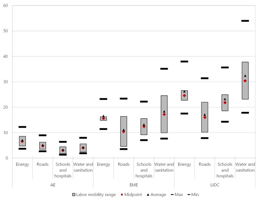
Figure 1. Job Content per US$1 Million of Additional Investment

 Notes: The figure shows the estimates of the job content of US$1 million of investment for
 different sectors and country groups based on regressions of employment on revenues
 over 1999–2017, covering 47,580 observations for 5,679 privately owned and state-owned
 enterprises. The stripped bar and the red rhombus represent the labor mobility range and
 midpoint estimate, respectively, for medium labor intensity. Labor mobility is the easiness of
 moving across companies within sectors (given by the point estimates in Table 3) and labor
 intensity is the path-through share to the supply chain in the sector (parametrized between
 35 and 65 percent). The thick horizontal dashes and the black triangle represent the overall
 maximum and minimum values and the average estimates, respectively, accounting for
 wide ranges of labor intensity. The estimates for low-income countries are extrapolated
 from the other estimates. AE: advanced economies; EME: emerging market economies;
 LIDC: low-income developing economies.
 Source: Author’s own estimations based on Compustat and Orbis.

The employment impact for intermediate levels of labor mobility and labor intensity ranges from
3 jobs in the schools and hospitals to 6.6 jobs in electricity per million U.S. dollars of spending in
AEs and from 16 jobs in roads to 30.4 jobs in water and sanitation in LIDCs. Put differently, each
unit of public spending creates more direct jobs in electricity in high-income countries and more
jobs in water and sanitation in low-income countries.

Sustainable “green” investment could create more jobs than traditional investment (Garrett-
Peltier, 2017; IMF, 2019; Allan and others, 2020; and Coalition of Finance Ministers for Climate
Action, 2020). Policymakers and scholars have advocated for a green recovery in the wake of the
Global Financial Crisis (Houser, Mohan, and Heilmayr, 2009; and Jacobs, 2012). The Great
Lockdown is calling anew for similar measures (Allan and others, 2020 and Coalition of Finance
Ministers for Climate Action, 2020). Jobs created in the renewable energy sector include solar

12

panel installation and building retrofitting, which have a high component of local labor. In
addition, many jobs in renewables do not require high educational attainment and have low
barriers to entry. In the United States, less than 20 percent of workers in clean-energy production
and energy-efficient occupations have college degrees (Muro and others, 2019). According to
the literature, job intensity—net of job losses in traditional industries—is estimated at 5–10 jobs
per US$1 million invested in green electricity, 2.4–12.5 jobs in efficient new buildings like schools
and hospitals, and 5.7–14 in green water and sanitation through efficient agricultural pumps and
recycling (Popp and others, 2020 and IEA, 2020). Altogether, the job creation multipliers per
US$1 million of green investment resemble the estimates for high labor intensity reported in
Table 4.

To complement our analysis and for additional robustness of our estimates, we compute the
impact of public spending on R&D on employment in R&D by type of recipient using a similar
approach of computing the employment elasticity to additional revenues. R&D is a smaller
component of public investment, which goes primarily to the government institutions and higher
education, and unlike other types of investment, employs high-skilled labor. These are higher-
quality jobs and are expected to increase, particularly in the health sector. Spending on R&D is
essential for long-term sustainable growth. We use OECD country-level data on R&D
disaggregated by recipient type and compute the pass-through from R&D spending to
employment in R&D. Overall, we collect 587 observations for 40 countries from 1999 to
2015 (with gaps).12 We convert spending in terms of annual shares of GDP to constant 2015 U.S.
dollars and run panel regressions analogous to those for public investment. Table 5 reports the
results of the regressions regarding R&D spending by recipient type in OECD countries. The
point estimates in Table 3 and Table 5 are in the same order of magnitude in terms of job
created by US$1 million, which validates the approach.

 Table 5. Job Content in R&D by Recipient Type

 (1) (2) (3) (4)
 Government Higher Education Business Non-Profit
 Spending in R&D (US$ million) 4.837*** 10.99*** 10.55** 4.477**
 (1.281) (3.970) (4.609) (2.020)
 Country fixed effects Yes Yes Yes Yes
 Cluster at country level Yes Yes Yes Yes
 Observations 409 405 414 287
 R-squared 0.690 0.425 0.635 0.331
 Number of clusters 36 36 37 25

Notes: This table presents the results of panel regressions of employment on spending in R&D in millions of
2015 U.S. dollars in OECD countries. The models correspond to recipients of R&D financing: government, higher
education, business, and private non-profit. The sample data is 1999-2015. Heteroskedasticity-robust standard
errors clustered at the country level are reported in parenthesis; *, **, and *** denote significance at 10, 5, and
1%, respectively.
Source: Author’s calculations.

12We exclude the blurry “intramural” category, which includes all expenditures for R&D performed within a
statistical unit or sector of the economy during a specific period, whatever the source of funds.

13

Government R&D generates an estimated 4.8 jobs in R&D per US$1 million invested. Higher
education R&D is nearly twice higher, possibly because it focuses on fundamental research and
requires less capital than government R&D, which in turn focuses often on capital-intensive
experimental and military applications (Chapter 8 in OECD, 2015).13 However, spending on higher
education R&D only accounts on average for 0.36 percent of GDP (about 20 percent of total
R&D spending) and the government R&D for 0.22 percent of GDP (about 13 percent of total
R&D spending). The largest R&D spending was carried by business for a total of 1.1 percent of
GDP and 61 percent of total spending in R&D.

Basic R&D is long-term and is primarily financed by the public sector, while the private sector
finances mainly applied R&D, which is medium-term at best. The job content of green R&D is
estimated at 3–8 jobs per US$1 million of investment (IEA, 2020); i.e., green R&D is not more
costly than conventional R&D and can have a lasting long-term impact.

Data limitations prevents unfolding the labor impact of different wage levels, full versus part-
time jobs, and types and degrees of green investment. The elasticity of job creation to wages is
estimated at the income level group. To the extent that these dimensions are country- and firm-
specific, they are absorbed by the fixed effects.

 IV. WELFARE AND POLITICAL ECONOMY CONSIDERATIONS

Public investment alternatives are interlinked with institutional capacity and fiscal space. While
AEs have the human and physical capital needed and can borrow at record-low interest rates to
scale up public investment, most EMEs and LIDCs find themselves in much less favorable
situation. In these countries, public debt levels are significantly elevated, and the costs of
borrowing are much higher. Moreover, in EMEs and LIDCs public investment policies are subject
to significant political economy and capacity constraints and tradeoffs. We can identify three
relevant areas for the debate on public investment in infrastructure.

State-own enterprises (SOEs), which often undertake public investment projects, have on average
higher job intensity than private firms (IMF, 2020a). SOEs operate in virtually every country, most
commonly in sectors such as public utilities, energy, transportation, and banking. In OECD
counties, SOEs represent, on average, 4.7 percent of the labor force, compared to 15.8 percent by
the general government (OECD, 2013). In some OECD countries, SOEs employ particularly large
parts of the non-agricultural workforce: e.g., Norway 9.6 percent, Latvia 6.7 percent, Estonia
4.8 percent, Hungary 4.2 percent, France 3.5 percent, Finland 3.5 percent, the Czech Republic
3.4 percent, the Slovak Republic 3.1 percent, and Italy 3.1 percent (OECD, 2017). Job intensity for
SOEs is found to be 30 percent higher than for their private counterparts (Baum and others,
2019). Possible explanations for this finding are that SOEs tend to be larger and have an implicit
employment remit. This result is especially important in EMEs and LIDCs, where SOEs account for
more than half of all infrastructure project commitments (IMF, 2020a) and often employ large
parts of the workforce.

13 See, also, Sargent Jr. (2020).

14

Public-private initiatives are not a panacea when the fiscal space to undertake public investments
is limited. First, public-private partnerships are not “free money” from the private sector to ease
public-sector financing. The private sector has a pecking order of projects where to invest driven
by profitability and enforcement of property rights. Second, fiscal capacity tends to be correlated
with state capacity (Besley and Persson, 2010 and Moszoro and others, 2015). The public and
private sectors are complementary in infrastructure when there is enough state capacity to
provide effective regulation and safeguard property rights (Besley and Persson, 2009). Third, if
there is sufficient fiscal space and state capacity, the private sector can contribute (in particular
cases) with superior technology and efficient management (Moszoro, 2018); if there is no fiscal
space, the private sector is also likely to be constrained in that jurisdiction, and it is unlikely that
the external private capital will solve institutional and financing deficiencies.

Policies on greening the recovery ought to be carefully designed to avoid backlash (Barbier,
2010). Clean-energy infrastructure has been found to be labor intensive in the short term
(Garrett-Peltier, 2017), although not all green investments create jobs quickly (Popp and others,
2020). Some forms of green investment are also not job rich in the long term and require specific
skills: for example, windmills are capital intensive and produced in only a few countries. Whereas
green investment offers clear global welfare gains (Hicks-Kaldor efficiency), the distributional
effects and Pareto efficiency for low-income countries are debatable.

 V. DISCUSSION AND CONCLUSIONS

This paper makes the case that in addition to its primary goal of creating infrastructure public
investment can also support employment. The emphasis on job creation is particularly relevant
during these unprecedented times that has had a dramatic impact on labor markets. We present
an innovative approach to measure the employment impact of public investment, which are
carried through sector-specific construction companies. We compute the employment effect of
US$1 million of spending by sector and country income group using a rich panel dataset with
firm-level data of construction companies from 1999 to 2017. Extrapolating our results to all AEs
and EMEs suggest that an increase in public investment equivalent to 1 percent of GDP could
directly create more than seven million jobs in AEs and EMEs through its direct employment
effects alone (i.e., about 5.4 percent of the full-time equivalent jobs lost in 2021 relative to fourth
quarter of 2019; ILO 2021, January). This number is obtained by applying: (i) a job content of
4.9 per US$1 million invested for AEs (unweighted average) to an increase in investment worth
1 percent of GDP in AEs (ca. US$500 billion in 2020; cf. Appendix 1) and (ii) a job content of
14.8 per US$1 million for emerging markets (similarly to AEs) to 1 percent of the GDP of EMEs
(ca. US$320 billion). The impact could be higher for green investment and for investments in
R&D with a higher labor intensity.

These numbers may underestimate job creation of public investment because of several factors
that go beyond the scope of the data, including:

 a) Firms with less than five observations are excluded. Thus, the analysis misses the
 employment increase in cyclical companies that are formed during fiscal expansion and
 disappear in times of fiscal consolidation, and which likely have higher elasticity between
 revenue and employment.

15

 b) The effects in LIDCs of additional employment are linearly extrapolated from AEs and
 EMEs. This relationship may arguably be convex: i.e., the impact on employment is likely
 increase exponentially the lower the country’s income per capita, as infrastructure
 development is more labor-intensive and the labor force is less specialized, and thus
 more fungible, in LIDCs (Tanzi, 2019).
 c) The indirect labor impact and spillovers (including Keynesian multiplier effects into other
 sectors of the economy) are not included. The IMF (2020b) estimates that a 1 percent of
 GDP increase in public investment in AEs and EMEs has the potential to create, directly
 and indirectly, between 20 and 33 million jobs.
 d) These estimates are pooled and do not distinguish between new projects and
 maintenance, or between skilled and unskilled labor. Ceteris paribus, maintenance
 projects and projects with a higher unskilled labor component would create more jobs
 than estimated here.

On the other hand, the job creation estimates may be overstated by the degree of waste from
budget allocations to actual contracted public investment. The Public Investment Management
Assessment (PIMA) database—which currently covers a cross-section of over 60 countries; see
IMF, 2015; IMF, 2018; and IMF’s web page on PIMA14—can serve as a tentative first approach to
correct for this upward bias.

Policies that provide preference for particular sectors in the short term may have longer-term
implications. For example, a preference for public works in roads may prevent investment in
electricity necessary for digital infrastructure. The estimates presented in Table 4 can serve as a
tool for policymakers to assess the employment impact and trade-offs of alternative uses of fiscal
space between short-term current and long-term capital spending, and between social and
physical capital sectors. They also quantify the enhancing employment impact of higher labor
mobility (e.g., through training and flexible arrangements) and higher labor content (e.g., in
infrastructure maintenance and green investment).

Future extensions of this work include the quantification of employment impact by country, in
digital infrastructure, and—inasmuch as the industrial classification evolves to encompass this
distinction—by green versus brown investment.

14Cf. https://infrastructuregovern.imf.org/content/PIMA/Home/PimaTool/What-is-PIMA.html (accessed February
2021).

16

 Appendix 1. Employment and GDP in Advanced Economies and Emerging Market
 Economies

This appendix contains the list of countries (classified by level of income), the employment in
millions of employees, and the GDP in billions of U.S. dollars. The sample includes firm-level data
from 38 advanced economies and 63 emerging market economies, for a total of 101 economies
representing 95 percent of the global GDP.

 Employment GDP
 Country Income level
 (millions) (US$ billions)
 Albania Emerging Market Economy 1.1 15.4
 Algeria Emerging Market Economy 11.1 172.8
 Argentina Emerging Market Economy 17.1 445.5
 Armenia Emerging Market Economy 1.6 13.4
 Azerbaijan Emerging Market Economy 5.0 47.2
 Bahamas, The Emerging Market Economy 0.2 12.7
 Bahrain Emerging Market Economy 0.9 38.2
 Barbados Emerging Market Economy 0.1 5.2
 Belarus Emerging Market Economy 4.3 62.6
 Belize Emerging Market Economy 0.2 2.0
 Bolivia Emerging Market Economy 5.6 42.4
 Bosnia and Herzegovina Emerging Market Economy 1.0 20.1
 Botswana Emerging Market Economy 1.5 18.7
 Brazil Emerging Market Economy 92.1 1,847.0
 Brunei Darussalam Emerging Market Economy 0.2 12.5
 Bulgaria Emerging Market Economy 3.1 66.2
 Cabo Verde Emerging Market Economy 0.3 2.0
 Chile Emerging Market Economy 8.6 294.2
 China Emerging Market Economy 775.3 1,4140.2
 Colombia Emerging Market Economy 22.9 327.9
 Costa Rica Emerging Market Economy 2.3 61.0
 Croatia Emerging Market Economy 1.4 60.7
 Dominican Republic Emerging Market Economy 4.6 89.5
 Ecuador Emerging Market Economy 7.5 107.9
 Egypt Emerging Market Economy 25.9 302.3
 El Salvador Emerging Market Economy 2.8 26.9
 Hungary Emerging Market Economy 4.5 170.4
 India Emerging Market Economy 32.0 2,935.6
 Indonesia Emerging Market Economy 127.1 1,111.7
 Iran Emerging Market Economy 25.1 458.5
 Jamaica Emerging Market Economy 1.2 15.7
 Jordan Emerging Market Economy 1.8 44.2
 Kazakhstan Emerging Market Economy 8.9 170.3
 Kuwait Emerging Market Economy 2.7 137.6
 Malaysia Emerging Market Economy 15.0 365.3
 Mauritius Emerging Market Economy 0.5 14.4
 Mexico Emerging Market Economy 54.4 1,274.2
 Mongolia Emerging Market Economy 1.3 13.6
 Morocco Emerging Market Economy 11.2 119.0
 North Macedonia Emerging Market Economy 0.8 12.7
 Oman Emerging Market Economy 2.3 76.6
 Pakistan Emerging Market Economy 59.8 284.2
 Panama Emerging Market Economy 1.9 68.5
 Peru Emerging Market Economy 16.9 229.0
 Philippines Emerging Market Economy 42.1 356.8
 Poland Emerging Market Economy 16.5 565.9
 Qatar Emerging Market Economy 2.2 191.8
 Romania Emerging Market Economy 8.8 243.7

17

 Employment GDP
 Country Income level
 (millions) (US$ billions)
 Russia Emerging Market Economy 72.7 1,637.9
 Serbia Emerging Market Economy 2.3 51.5
 Seychelles Emerging Market Economy 0.0 1.6
 South Africa Emerging Market Economy 16.6 358.8
 Suriname Emerging Market Economy 0.1 3.8
 Thailand Emerging Market Economy 37.4 529.2
 Trinidad and Tobago Emerging Market Economy 0.6 22.6
 Tunisia Emerging Market Economy 3.5 38.7
 Turkey Emerging Market Economy 28.2 743.7
 Turkmenistan Emerging Market Economy 2.5 46.7
 Ukraine Emerging Market Economy 16.4 150.4
 United Arab Emirates Emerging Market Economy 7.7 405.8
 Uruguay Emerging Market Economy 1.7 59.9
 Venezuela Emerging Market Economy 8.4 70.1
 Vietnam Emerging Market Economy 58.3 261.6
 Australia Advanced Economy 12.9 1,376.3
 Austria Advanced Economy 4.4 447.7
 Belgium Advanced Economy 4.9 517.6
 Canada Advanced Economy 19.0 1,730.9
 Cyprus Advanced Economy 0.4 24.3
 Czech Republic Advanced Economy 5.3 247.0
 Denmark Advanced Economy 2.9 347.2
 Estonia Advanced Economy 0.7 31.0
 Finland Advanced Economy 2.6 269.7
 France Advanced Economy 25.6 2,707.1
 Germany Advanced Economy 42.0 3,863.3
 Greece Advanced Economy 3.9 214.0
 Hong Kong SAR Advanced Economy 3.9 373.0
 Iceland Advanced Economy 0.2 23.9
 Ireland Advanced Economy 2.3 384.9
 Israel Advanced Economy 4.0 387.7
 Italy Advanced Economy 23.3 1,988.6
 Japan Advanced Economy 67.4 5,154.5
 Korea Advanced Economy 26.9 1,629.5
 Latvia Advanced Economy 0.9 35.0
 Lithuania Advanced Economy 1.4 53.6
 Luxembourg Advanced Economy 0.5 69.5
 Macao SAR Advanced Economy 0.4 55.1
 Malta Advanced Economy 0.2 14.9
 Netherlands Advanced Economy 8.9 902.4
 New Zealand Advanced Economy 2.7 204.7
 Norway Advanced Economy 2.7 417.6
 Portugal Advanced Economy 5.0 236.4
 Puerto Rico Advanced Economy 1.0 99.9
 Singapore Advanced Economy 3.7 362.8
 Slovak Republic Advanced Economy 2.4 106.6
 Slovenia Advanced Economy 1.0 54.2
 Spain Advanced Economy 19.8 1,397.9
 Sweden Advanced Economy 5.1 528.9
 Switzerland Advanced Economy 5.0 715.4
 Taiwan Province of China Advanced Economy 11.5 586.1
 United Kingdom Advanced Economy 32.8 2,743.6
 United States Advanced Economy 156.9 21,439.5
 Sum 2,204.4 83,218.7

Source: WEO and IMF.

REFERENCES

Aizer, Anna, Shari Eli, Adriana Lleras-Muney, and Keyoung Lee, 2020, “Do Youth Employment
 Programs Work? Evidence from the New Deal,” NBER Working Paper No. 27103
 (Cambridge, Massachusetts: National Bureau of Economic Research).
Allan, Jennifer, Charles Donovan, Paul Ekins, Ajay Gambhir, Cameron Hepburn, David Reay, Nick
 Robins, Emily Shuckburgh, and Dimitri Zenghelis, 2020, “A Net-Zero Emissions Economic
 Recovery from COVID-19,” Smith School Working Paper 20-01 (Oxford Smith School of
 Enterprise and the Environment).
Auerbach, Alan J., and Yuriy Gorodnichenko, 2013, “Output Spillovers from Fiscal Policy,”
 American Economic Review, Vol. 103, No. 3, pp.141–46.
Barbier, Edward, 2010, “Green Stimulus, Green Recovery and Global Imbalances,” World
 Economics Journal, Vol. 11, No. 2, pp.149–77.
Baum, Anja, Clay Hackney, Paulo Medas, and Mouhamadou Sy, 2019, “Governance and State-
 Owned Enterprises: How Costly is Corruption?,” IMF Working Paper No. 19/253
 (Washington: International Monetary Fund).
Besley, Timothy, and Torsten Persson, 2009, “The Origins of State Capacity: Property Rights,
 Taxation, and Politics,” American Economic Review, Vol. 99, No. 4, pp.1218–44.
______, 2010, “State Capacity, Conflict, and Development,” Econometrica, Vol. 78, No. 1, pp.1–34.
Blanchard, Olivier J., and Lawrence H. Summers, 1986, “Hysteresis and the European
 Unemployment Problem,” NBER Working Paper Series No. 1950, pp.15–78 (Cambridge,
 Massachusetts: National Bureau of Economic Research).
Coalition of Finance Ministers for Climate Action, The, 2020, “Better Recovery, Better World:
 Resetting Climate Action in the Aftermath of the COVID-19 Pandemic,” (Washington: The
 World Bank Group).
Emrath, Paul, 2015, “Subcontracting: Three-Fourths of Construction Cost in the Typical Home,”
 National Association of Home Builders (NAHB) Special Studies Series (Washington:
 National Association of Home Builders).
Garin, Andrew, 2019, “Putting America to Work, Where? Evidence on the Effectiveness of
 Infrastructure Construction as a Locally Targeted Employment Policy,” Journal of Urban
 Economics, Vol. 111, pp.108–31.
Garrett-Peltier, Heidi, 2017, “Green versus brown: Comparing the employment impacts of energy
 efficiency, renewable energy, and fossil fuels using an input-output model,” Economic
 Modelling, Vol. 61, pp. 439–47.
Gaspar, Vitor, David Amaglobeli, Mercedes Garcia-Escribano, Delphine Prady, and Mauricio Soto,
 2019, “Fiscal Policy and Development: Human, Social, and Physical Investments for the
 SDGs,” Staff Discussion Notes No. 19/03 (Washington: International Monetary Fund).
Houser, Trevor, Shashank Mohan, and Robert Heilmayr, 2009, “A Green Global Recovery?
 Assessing US Economic Stimulus and the Prospects for International Coordination,” Policy
 Brief 09-3, (Washington: Peterson Institute for International Economics).

19

International Energy Agency (IEA), 2020, “Sustainable Recovery,” World Energy Outlook Special
 Report (Paris, France).
International Labour Organisation, 2021, “ILO Monitor: COVID-19 and the World of Work. 7th
 Edition,” Briefing note, (Geneva: International Labour Organization).
International Monetary Fund, 2015, “Making Public Investment More Efficient,” IMF Policy Paper
 (Washington: International Monetary Fund).
______, 2018, “Public Investment Management Assessment—Review and Update,” IMF Policy
 Paper (Washington: International Monetary Fund).
______, 2019, “How to Mitigate Climate Change,” October 2019 Fiscal Monitor (Washington:
 International Monetary Fund).
______, 2020a, “Policies to Support People During the COVID-19 Pandemic,” April 2020 Fiscal
 Monitor (Washington: International Monetary Fund).
______, 2020b, “Policies for the Recovery,” October 2020 Fiscal Monitor (Washington: International
 Monetary Fund).
______, 2021, “A Fair Shot,” April 2021 Fiscal Monitor (Washington: International Monetary Fund).
Jacobs, Michael, 2012, “Green Growth: Economic Theory and Political Discourse,” Working Paper
 No. 92 (London: Grantham Research Institute on Climate Change and the Environment at
 The London School of Economics and Political Science).
Kézdi, Gabor, 2004, “Robust Standard Error Estimation in Fixed-Effects Panel Models,” Hungarian
 Statistical Review, Special Number 9, pp. 96–116.
Moszoro, Mariano, Gonzalo Araya, Fernanda Ruiz-Nuñez, and Jordan Schwartz, 2015, “What
 Drives Private Participation in Infrastructure Developing Countries?,” in Public Private
 Partnerships for Infrastructure and Business Development, ed. by Stefano Caselli, Guido
 Corbetta, and Veronica Vecchi (New York: Palgrave Macmillan).
Moszoro, Mariano, 2018, “Public–Private Monopoly,” The B.E Journal of Economic Analysis &
 Policy, Vol. 18, No. 2, pp.1–15.
Mummolo, Jonathan, and Erik Peterson, 2018, “Improving the Interpretation of Fixed Effects
 Regression Results,” Political Science Research and Methods, Vol. 6, No. 4, pp. 829–35.
Muro, Mark, Adie Tomer, Ranjitha Shivaram, and Joseph W. Kane, 2019, Advancing Inclusion
 through Clean Energy Jobs. Metropolitan Policy Program (Washington: Brookings
 Institution).
Organization for Economic Cooperation and Development, 2013, “Employment in General
 Government and Public Corporations,” in Government at a Glance 2013 (Paris: OECD
 Publishing).
______, 2015, “Government R&D”, Chapter 8 in Frascati Manual 2015: Guidelines for Collecting and
 Reporting Data on Research and Experimental Development,” The Measurement of
 Scientific, Technological and Innovation Activities (Paris: OECD Publishing).
______, 2017, The Size and Sectoral Distribution of State-Owned Enterprises (Paris: OECD
 Publishing).

20

Papanikolaou, Dimitris, and Lawrence D.W. Schmidt, 2020, “Working Remotely and the Supply-
 side Impact of Covid-19,” NBER Working Paper No. 27330 (Cambridge, Massachusetts:
 National Bureau of Economic Research).
Popp, David, Francesco Vona, Giovanni Marin, and Ziqiao Chen, 2020, “The Employment Impact
 of Green Fiscal Push: Evidence from the American Recovery Act,” NBER Working Paper
 No. 27321 (Cambridge, Massachusetts: National Bureau of Economic Research).
Ramey, Valerie A. , 2020, “The Macroeconomic Consequences of Infrastructure Investment,” NBER
 Working Paper No. 27625 (Cambridge, Massachusetts: National Bureau of Economic
 Research).
Sargent Jr., John F., 2020, “Federal Research and Development (R&D) Funding: FY2020,” CRS
 Report R45715 (Washington: Congressional Research Service).
Tanzi, Vito, 2019, “The Limits of Stabilization Policies,” Acta Oeconomica, Vol. 69, pp. 141–51.
______, and Hamid Davoodi, 1998, “Corruption, Public Investment, and Growth,” in The Welfare
 State, Public Investment, and Growth, ed. by Hirofumi Shibata and Toshihiro Ihori (Tokyo:
 Springer).
Wilson, Daniel J., 2012, “Fiscal Spending Jobs Multipliers: Evidence from the 2009 American
 Recovery and Reinvestment Act,” American Economic Journal: Economic Policy, Vol. 4, No.
 3, pp. 251–82.
Wooldridge, Jeffrey M., 2003, “Cluster-Sample Methods in Applied Econometrics,” American
 Economic Review, Vol. 93, No. 2, pp.133–38.
Yackovlev, Irene, Zuzana Murgasova, Fei Liu, Gohar Minasyan, and Ke Wang, 2020, “How to
 Operationalize IMF Engagement on Social Spending during and in the aftermath of the
 COVID-19 Crisis,” IMF How-To Note No. 20/02 (Washington: International Monetary
 Fund).