The effect of straight chimney temperature on pollutant dispersion
←
→
Page content transcription
If your browser does not render page correctly, please read the page content below
E3S Web of Conferences 234, 00009 (2021)                                                     https://doi.org/10.1051/e3sconf/202123400009
ICIES 2020

    The effect of straight chimney temperature on pollutant
    dispersion
    Fida Zair1,*, Mhamed Mouqallid2, and El houssine Chatri1
    1 Laboratory of Atomic, Mechanical, Photonic and Energetic, Faculty of Sciences, Moulay Ismail University, Physics Departement,
    Meknes, Morocco
    2 Department of Energy, ENSAM Meknes, Moulay Ismail University, Meknes, Morocco

                  Abstract. Air pollution is considered one of the most important contemporary problems that threaten a
                  person's life and environment. Among the major sources of air pollution are pollutants emitted from
                  smokestacks. The objective of this work is to numerically study the dispersion of a pollutant ejected from a
                  chimney into an air stream. The mass, momentum and energy conservation equations are solved using the
                  finite volume method (MFV) and numerical simulations are performed using Ansys Fluent CFD software.
                  Two case studies were discussed: The first case study is to study the influence of the direction of the wind
                  speed and in the last case study, the temperature evolution on the dispersion of the ejected plume particles.
                  The study demonstrated the extent of the dispersion in relation to these two parameters. The results obtained
                  confirm the need to improve filtering systems in order to reduce the risks attributed to discharges and to
                  propose solutions to manage the effect of these discharges on the environmental population.

  1 Introduction                                                        chimneys of a cement plant. The study is conducted in
                                                                        numerical form and aims to determine the effects of the
  Air pollution is a very complex phenomenon given the                  following factors (wind speed, stack height,
  diversity of pollutants, their combination and their                  environmental roughness) on the diffusion of particles in
  modification in the atmosphere. The evolution of these                the ejected plume.
  contaminants is difficult to understand rigorously, this                  This paper is founded on earlier work by Smith and
  complexity contributes to heightened concerns about air               Frankenberg [3] which showed that stack height
  quality. Emissions from industrial chimneys are a major               influences dispersion under thermal inversion (when a
  source of air pollution and their dispersion depends on               pollutant is emitted from a low stack opening below the
  several parameters in particular.                                     thermal inversion layer, there is an accumulation of the
      Previous work in this area has focused on                         thermal inversion layer below, but if the stack opens
  determining the influence of these parameters on the                  above it, the pollutants diffuse normally).
  dispersion phenomenon. A study on the parameters                          Wilson [4] and Vincent's [5] studies of the
  influencing the dispersion of gaseous pollutants was                  atmospheric boundary layer. They highlighted the
  carried out by Diaf and Bouchaour [1] in which they                   influence of obstacles on the dispersion of pollutants.
  stated that the dispersion of pollutants in the atmosphere            They found that the dispersion is more pronounced for
  is essentially carried out in the atmospheric boundary                larger injection ratios (R = (ejection velocity)⁄(wind
  layer: the most disturbed layer, constantly agitated by               speed)) and they found that the height reached by the
  turbulent movements. This dispersion is influenced by                 particles in the vicinity of the outlet is significant when
  several parameters such as wind speed, atmospheric                    R increases. When R is low (wind speed increases) the
  stability and thermal state.                                          dispersion of particles will be similarly low while the
      The results found show that the dispersion of gaseous             concentration is relatively high. The high crosswind
  pollutants through the atmosphere is very complex.                    speed favours dilution of the plume.
  Thus, an anticyclonic situation (very light winds) favours                In addition, stack elevation affects the dispersion of
  high levels of pollution because it leads to an                       releases. Ejection at a higher elevation generates a larger
  accumulation of gases.                                                plume that promotes dilution. The higher the height, the
      The inversion of the vertical thermal gradient has the            further away the maximum concentration moves and
  same consequences. In the opposite, a low-pressure                    leaves the domain.
  situation (i.e. more sensitive winds) allows a better                     Menaouer [6] studied a numerical model of the
  dilution of pollutants in the atmosphere.                             evolution of the dispersion of pollutants emitted by a
      Benkoussas and Bouhdjar [2] conducted a study on                  stack. This work is a numerical approach employed to
  the atmospheric dispersion of effluents emitted by the                define the fields of continuous or instantaneous

    *
        Corresponding author: f.zair@edu.umi.ac.ma

© The Authors, published by EDP Sciences. This is an open access article distributed under the terms of the Creative Commons Attribution
License 4.0 (http://creativecommons.org/licenses/by/4.0/).
E3S Web of Conferences 234, 00009 (2021) ICIES’2020 https://doi.org/10.1051/e3sconf/202123400009
ICIES 2020
dispersion of pollutants by industrial stacks, the results found near buildings with CFD simulations. They further
of which help in decision-making and determine the risk indicated that dispersion could be artificially increased
areas, therefore, the choice of a plant location. This by reducing the Sct.
research also permits to define the effect of different Tominaga and Stathopoulos [11] investigate different
physical parameters on the dispersion phenomenon, for models of airflow turbulence and pollutant dispersion on
example wind velocity and the roughness of the an isolated cubic obstacle. They further discovered that
environment. the standard k-ɛ model did not predict concentrations
Numerical simulations of atmospheric dispersion because it does not replicate the basic components of
under the ANSYS FLUENT 12.1 allow to plot the flow flow structures, for example, opposite flow on the roof
characteristics (velocities, concentrations, etc.) and to of a building. The k-ɛ RNG model and the k-ɛ Realizable
detect the characteristics of the plume in a neutral model were in accord with the experimental data for Sct
situation. The results obtained are plotted and are in very = 0.3. This allowed the authors to confirm that the
good accordance with those in the literature. underestimation of turbulent pulse scattering in the wind
Flowe and Kumar [7] conducted a parametric study flow could be compensated for by a lower Sct value.
to determine the length of the recirculation cavity The objective of our paper is to study the influence of
according to the ratio of the width of the building to the some parameters on the dispersion of pollutants emitted
height of the building, both at the front and at the back of by straight chimneys: wind speed direction and jet
the building. The main purpose of this investigation was temperature.
to assess the viability of utilizing a three-dimensional k-ε
digital model to model airflow beyond the geometry of
the building and chimney. The dispersive data collected 2 Methodology
was then used to determine new correlations between the
ratio of building width to height, the size of the 2.1. Governing Equation
recirculation cavity and the medium concentration in the
subsequent recirculation cavity of the building. Considering the flow from a chimney. The chimney
Liu and Ahmadi [8] have studied the movement, emits a mixture of air and smoke at Uchimney speed and
dispersion and deposition of particles in the vicinity of a Tchimney temperature. This plume is subjected to a wind
building using a Lagrangian particle survey approach. speed of Uwind, the ambient temperature is T wind.
The computational model used reported the forces of The governing equations are based on the continuity
train and uplift acting on the particles as in addition to and the momentum equations in steady state. The
the influence of Brownian motion and the effects of fluctuating velocity components were averaged
gravitational sedimentation. A point source of helium according to Reynolds Navies- Stokes decomposition
was selected as the contaminant source, and the helium RANS were U i ui ui' That maybe written for the
concentration in the posterior plane of the building,
mean field as:
perpendicular to the direction of air flow, was evaluated.
u i
The results found that the diffusion and deposition of 0 (1)
particles of 0.01 μm and 1 μm were comparable, and that x i
the gravitational force had a significant impact on the
deposition rate of particles of 10 μm. Comparison of the
u i 1 P u i
results with the available data revealed agreement on the uj
u i' u 'j (2)
average airflow and the average gas concentration. x j x i x j x j
Olvera et al [9] studied the posterior recirculation
cavity of a cubic building at using a commercial CFD U U j 2
code and the turbulence model k-ɛ RNG. They found With: u i' u 'j t i ij (3)
x j x i 3
that plume flotation affects the size and form of the
cavity area of the flow profile and the concentrations
within this area. In their study report, the authors Where κ is the turbulent kinetic energy defined by:
recommended including this effect in the plume folding
algorithm to improve the accuracy of far-field 1
concentration distribution modelling results. u i' u 'j (4)
2
This would be essential for accident investigations,
when accurate predictions of near-field concentration
fluctuations near the source over short periods of time The term u i' u 'j identifies the Reynolds stresses
are required. tensor. This additional term is take into account through
DiSabatino et al [10] studied the effect of the Sct on new equations that require closure or turbulence models.
airflow in a small building configuration and on the
dispersion of pollutants in urban canyons. To this end,
they compared the standard k-ɛ model with the ADMS- 2.2. Turbulence Modeling
Urban atmospheric dispersion model. Like previous The mathematical models used are turbulence models
researchers, they found that concentrations were with two equations of the first order (κ - ε standard, κ - ε
overestimated in urban canyons, a phenomenon they RNG, κ - ε Realizable, κ - ω and κ - ω SST) and the
attributed to the low values for turbulent kinetic energy
2
E3S Web of Conferences 234, 00009 (2021) ICIES’2020 https://doi.org/10.1051/e3sconf/202123400009
ICIES 2020
second order RSM. All models are tested and give the motion quantity equation and the energy equation. For
same results when found, but in short, we just presented pressure-speed coupling, we adopted the SIMPLE
the RNG κ - ε model. algorithm, for coupling between the equations for
As introduced by Launder and Spalding [12], the conserving the amount of motion and the continuity
RNG κ - ε model were applied using the eddy viscosity equation.
νt model schemes given by: To complete the problem, in addition to the systems
of equations mentioned above, the boundary conditions
2 summarized in the following table (Table 1) must be
t C (5) taken into account:
Table 1. Boundary conditions
Where ɛ is the kinetic energy dissipation rate taken as:
2 Ui Chimney wall,
Chimney Wind
(6) ground
x 2j
For the RNG κ - ε model the turbulent kinetic energy κ U=0 U = Uwind U=0
Velocity
and the kinetic energy dissipation ε are given by the V = Uchimney V=0 V=0
following equations
Turbulent kinetic energy transport equation κ
∂T
Temperature T = Tchimney T = Twind =0
Ui ( eff ) P (7) ∂n
t x i x i x i
The kinetic energy dissipation equation ɛ
2
Ui ( eff ) C1P C 2 R
t x i x j x i
(8)
Ui U j Ui
With: P
t (9)
x j x i x j
With: Cν, Cɛ1 and Cɛ2 are the empirical coefficients and
σκ and σɛ are the turbulent Prandtl numbers for κ and ɛ
respectively. Rɛ is the additional term related to the shear
deformation velocity.
The constants of the RNG model are known.
3 Geometry of the Calculation Domain Figure 1. Geometry diagram
and Boundary Conditions
In Fig.1 we consider a straight chimney with a height h =
0,10 m and a diameter d = 0,01 m. The jet ejected from
the chimney and the transverse flow contain air, the ratio 4 Results and Interpretations
between the ejection velocity and that of the transverse
flow is equal to R = 1.6. The calculation range is wide
enough so that the boundaries of the range do not disturb 4.1. Validation of Results
the flow.
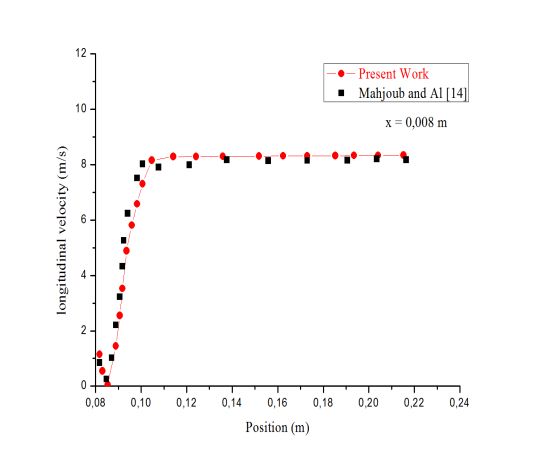
The results of the validation are plotted for longitudinal
The flow topology requires a very fine mesh in a
(U) velocity profiles using the same conditions of
large part of the domain. In order to obtain a precise
Mahjoub and Al [14]. The numerical simulation is tested
description of all variations, especially those closest to
for an incompressible and unsteady flow.
the chimney. We have adopted a non-uniform mesh size.
Figures 2-4 show the velocity profiles for different
To do this, the commercial code CFD ANSYS/FLUENT
cross-sections x (x = -0.005 m; x = 0 m and x = 0.008 m)
was used, which was able to simulate the dispersion
of the flow. These figures show a good agreement
phenomenon using the finite volume method presented
between the results found and those of Mahjoub and Al
by Patankar [13].
[14].
For the discretization schemes, we have adopted the
following schemes:
The "First Order Upwind" diagram for the turbulence
kinetic energy equations, the dissipation equation, the
3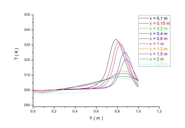
E3S Web of Conferences 234, 00009 (2021) ICIES’2020 https://doi.org/10.1051/e3sconf/202123400009
ICIES 2020
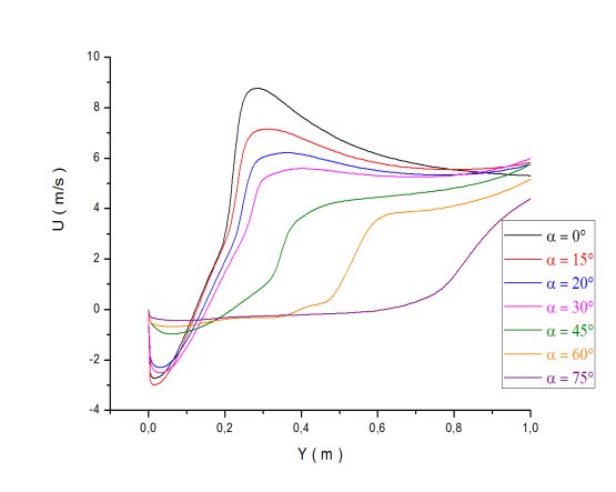
the stack). In Fig.5 and 6, we present the variation in
longitudinal and transverse velocity as a function of Y,
respectively.
It should be noted that the speed curve remains the
same for all seven values of α and that, the greater the
direction angle, the higher the dispersion of pollutants.
Figure 2. Longitudinal velocity profile for position
x = -0.005 m
Figure 6. Evolution of the longitudinal velocity at
x = 0.2 m for a straight chimney
Figure 3. Longitudinal velocity profile for position
x=0m
Figure 4. Evolution of the transverse velocity at
x = 0.2 m for a straight chimney
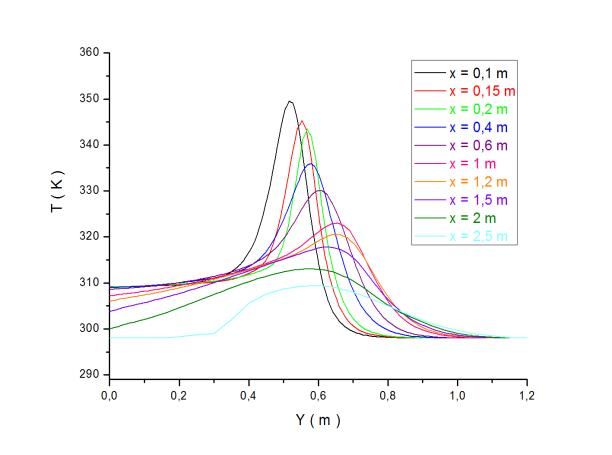
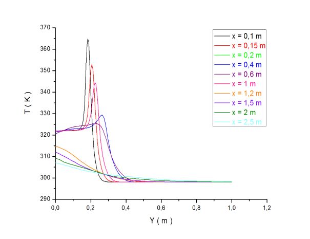
4.2.2 The Evolution of the Jet Temperature
This section keeps the same ratio of speeds R which is
equal to 1.6. We trace the evolution of the temperature
according to Y. To do this, one moves away from the
chimney each time by a distance x (x=0.2, 0.4, 0.6, 1.2, 2
Figure 5. Longitudinal velocity profile for position and 2,5 m) and one traces the value of the temperature
x = 0.008 m on function of Y.
For the curve 7, the temperature change starts from Y
4.2. Discussion = 0.1 m, which means that we do not have a decent
pollutant. All curves have the same speed but, when
4.2.1 The Effect of Wind Velocity Direction moving away from the stack, the maximum temperature
of the pollutant decreases. In addition, when the ejection
To study the influence of wind speed direction on temperature is increased, the maximum temperature
pollutant dispersion, the wind direction has been value increases.
changed (α = 0°, α=15°, α=20°, α=30°, α=45°, α=60°
and α=75°) and for the ejection speed will be fixed at 8
m/s, while the wind speed is equal to 5 m/s. Depending
on these directions, the dispersion results were obtained
in an area x = 0.2 m from the chimney (downstream of
4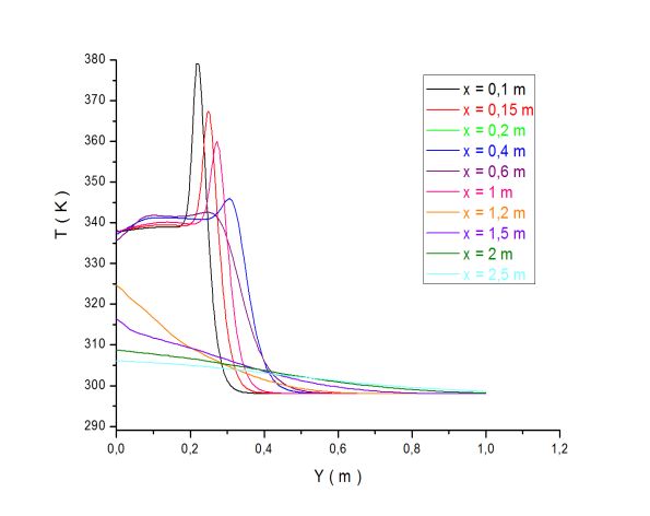
E3S Web of Conferences 234, 00009 (2021)                      ICIES’2020                     https://doi.org/10.1051/e3sconf/202123400009
ICIES 2020

                   Figure 7. Influence of temperature for different values of α and at each position of x (straight stack)

                                                                    5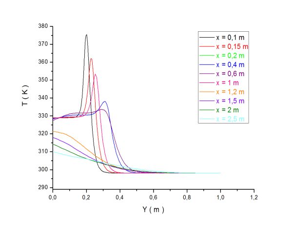
E3S Web of Conferences 234, 00009 (2021)                  ICIES’2020                   https://doi.org/10.1051/e3sconf/202123400009
ICIES 2020

                                                                     9.    H.A. Olvera, A.R. Choudhuri, W.W. Li . Effects of
                                                                           plume buoyancy and momentum on the near-wake
   5 Conclusions                                                           flow structure and dispersion behind an idealized
   In this work, a numerical simulation of the turbulent                   building. J Wind Eng Ind Aerodyn . 96:209-228
   flow from a straight chimney was performed. For this                    (2008).
   purpose, a 2D calculation code was used for an                    10.   S. DiSabatino et al . Simulations of pollutant
   incompressible fluid. This code is based on a finite                    dispersion within idealised urban-type geometries
   volume method to solve the complete Navier Stokes                       with CFD and integral models. Atmos Environ .
   equations was used in this study. We first showed the                   41:8316-8329 (2007).
   comparison between our results obtained digitally with            11.   Y. Tominaga & T. Stathopoulos . Numerical
   that of the literature in which a good agreement was                    simulation of dispersion around an isolated cubic
   illustrated.                                                            building: Comparison of various types of k-ε
       Second the results found allow to determine the                     models. Atmos Environ . 43:3200-3210 (2009).
   effect of the variation of several parameters on the flow         12.   B.E. Launder, D.B. Spaliding .The Numerical
   such as wind speed direction and jet temperature. It has                Computation of Turbulent Flows. Comput Methods
   been shown that the greater the angle of the wind                       Appl Mech Eng . 3:269-289 (1974).
   direction, the greater the dispersion of pollutants.
       We also note that the temperature of the jet ejected          13.   S.V. Patankar .Numerical heat transfer and fluid
   from the chimney has a great effect on the dispersion.                  flow. McGraw-Hill B Company, New York (1980).
   Indeed, the further away from the chimney the maximum             14.   S.N. Mahjoub, H. Mhiri, G. Le Palec, PH. Bournot.
   temperature of the pollutant decreases.                                 Experimental and numerical analysis of pollutant
       In future studies, it is important to study the                     dispersion from a chimney. Atmos Environ .
   relationship between the diameter of the chimney and the                39:1727-1738 (2005).
   dispersion of pollutants in the air. In addition, the study
   will be conducted under the variability of wind speed
   and direction.

   References
   1.   N. Diaf, M. Bouchaour, L. Merad, B. Benyoucef
        .Paramètres influençant la dispersion des polluants
        gazeux. RevEnergRen : ICPWE 139-142 (2003).
   2.   B. Benkoussas et al . Etude de la dispersion
        atmosphérique des effluents émis par les cheminées
        de la cimenterie de Meftah. J Sci Res N° 0 . 1:39-43
        (2010).
   3.   M.E. Frankenberg & T.T. Smith . Improvement of
        Ambient Sulfur Dioxide Concentrations by
        Conversion from Low to High Stacks. J Air Pollut
        Control Assoc . 25:595-601(1975).
   4.   D.J. Wilson . Turbulent dispersion in atmospheric
        shear flow and its wind tunnel simulation, Von
        Karman Institute for fluid dynamics, Technical note
        76. (1971).
   5.   J.H. Vincent . Model experiments on the nature of
        air pollution transport near buildings. Atmos
        Environ . 11:765-774 (1977).
   6.   M. Menaouer . Modélisation numérique de
        l’évolution de la dispersion des polluants émis par
        une cheminée. Université des Sciences et de la
        Technologie Mohammed BOUDIAF-Oran (2013).
   7.   A.C. Flowe, A. Kumar . Analysis of velocity fields
        and dispersive cavity parameters as a function of
        building width to building height ratio using a 3-D
        computer model for squat buildings. J Wind Eng Ind
        Aerodyn . 86:87-122 (2000).
   8.   C. Liu & G. Ahmadi . Transport and deposition of
        particles near a building model. Build Environ .
        41:828-836 (2006).

                                                                 6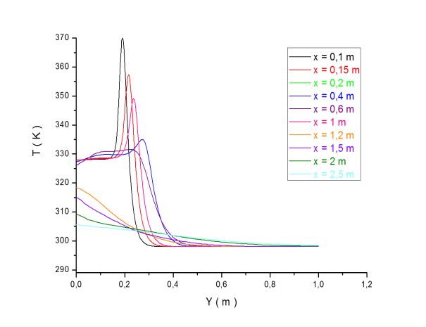
You can also read