The Great Gatsby Curve - Steven N. Durlauf, Andros Kourtellos, and Chih Ming Tan - Becker Friedman Institute
←
→
Page content transcription
If your browser does not render page correctly, please read the page content below
WORKING PAPER · NO. 2022-29

The Great Gatsby Curve
Steven N. Durlauf, Andros Kourtellos, and Chih Ming Tan
FEBRUARY 2022

                                                          5757 S. University Ave.
                                                              Chicago, IL 60637
                                                             Main: 773.702.5599
                                                               bfi.uchicago.edu
THE GREAT GATSBY CURVE
Steven N. Durlauf
Andros Kourtellos
Chih Ming Tan
February 2022
Durlauf thanks the Institute for New Economic Thinking and the Archbridge Foundation for
financial support. Tan thanks the Greg and Cindy Page Faculty Distribution Fund for financial
support.
© 2022 by Steven N. Durlauf, Andros Kourtellos, and Chih Ming Tan. All rights reserved. Short
sections of text, not to exceed two paragraphs, may be quoted without explicit permission
provided that full credit, including © notice, is given to the source.The Great Gatsby Curve
Steven N. Durlauf, Andros Kourtellos, and Chih Ming Tan
February 2022
JEL No. D3,H0,J0,R0
ABSTRACT
This paper provides a synthesis of theoretical and empirical work on the Great Gatsby Curve, the
positive empirical relationship between cross-section income inequality and persistence of
income across generations. We present statistical models of income dynamics that mechanically
give rise to the relationship between inequality and mobility. Five distinct classes of theories,
including models on family investments, skills, social influences, political economy, and
aspirations are developed, each providing a behavioral mechanism to explain the relationship.
Finally, we review empirical studies that provide evidence of the curve for a range of contexts
and socioeconomic outcomes as well as explore evidence on mechanisms.
Steven N. Durlauf Chih Ming Tan
University of Chicago Department of Economics
Harris School of Public Policy College of Business and Public Administration
1307 E. 60th Street University of North Dakota
Chicago, IL 60637 Gamble Hall Room 290
and NBER 293 Centennial Drive Stop 8369
durlauf@gmail.com Grand Forks, ND 58202-8369
chihmingtan@gmail.com
Andros Kourtellos
Department of Economics
University of Cyprus
P.O. Box 20537
CY-1678 Nicosia
CYPRUS
andros@ucy.ac.cyI. Introduction
One of the most visible stylized facts in contemporary inequality research is the
association, across national economies, between measures of cross-section income
inequality and intergenerational mobility or persistence. At the cross-country level, this
relationship was recognized early by Hassler, Mora, and Zeira (2007), Andrews and Leigh
(2009), Björklund and Jäntti (2009), and Corak (2006,2013a,b), whose work has received
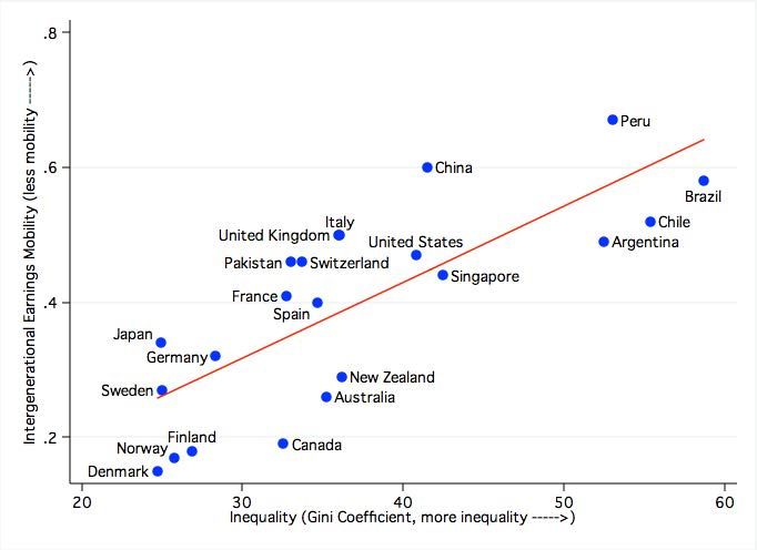
particular attention. Figure 1, taken from Corak (2013b), illustrates the relationship, which
describes a positive association between inequality, measured by a country’s Gini
coefficient, and persistence, measured by the intergenerational elasticity of income (IGE)1
linking parent and offspring permanent incomes. Krueger (2012), based on Corak’s work,
dubbed the positive relationship between inequality and persistence, the Great Gatsby
Curve (GGC), and introduced it into popular and policy discussion.
The prominence of the curve in policy debates derives from several reasons. First,
it suggests that a society can simultaneously pursue equality of outcomes (measured by
cross-section differences) and equality of opportunity (measured by mobility). Second,
and specific to the American context, the curve challenged the longstanding idea that the
US has, in contrast to other societies, made choices on socioeconomic structure that
accept unequal outcomes in order to produce equal opportunities; i.e., Americans believe
in the proverbial American Dream. Longstanding social science traditions have argued
that this view of opportunity is integral to the American character. For example, Potter’s
classic (1954) discussion of how American abundance created a distinct national
character is based on the idea that America offered qualitatively greater socioeconomic
opportunities than did Europe, at least for white males. Lipset (1994) argues that an
important dimension of American exceptionalism is a commitment to meritocracy, which
is intertwined with the belief that America offers ample opportunities that are not
determined by family background. Fischer (2010) suggests that a key feature of the
American character is voluntarism, which is described by:
1The IGE is defined by equation (1) below.
1The first key element of voluntarism is believing and behaving as if each
person is a sovereign individual, unique, independent, self-reliant, self-
governing, and ultimately self-responsible…The second key element is
believing and behaving as if individuals succeed through fellowship…in
sustaining voluntary communities…In a voluntaristic culture people assume
that they control their own fates and are responsible for themselves. (10)
Since the GGC links inequality to limits in opportunity, it has been popularly regarded as
a challenge to American national myths.
The GGC also has normative implications. Much modern thought on equality of
opportunity and justice focuses on the role of individual responsibility in distinguishing just
versus unjust inequalities. Cohen (1989) famously argues that justice demands
equal access to advantage, where "advantage" is understood to include, but to
be wider than, welfare. Under equal access to advantage, the fundamental
distinction for an egalitarian is between choice and luck in the shaping of people's
fates. (907)
Roemer (1993,1998) elaborates on this approach and provides ways to operationalize
this form of just opportunity. Since parental socioeconomic status is an obvious case of
something for which children are not responsible, the extent to which inequality induces
intergenerational persistence means that cross-section inequality leads to injustices. To
the extent that intergenerational persistence generates cross-section inequality, this
inequality would therefore derive from unjust mechanisms 2.
The GGC has generated much research. On the theory side, the search for
mechanisms to explain the curve has involved understanding what sorts of
socioeconomic environments can produce a GGC within a given country across time. The
2The logic of responsibility sensitive egalitarianism must be adjudicated against other
social goods before drawing clear ethical conclusions. One clear issue involves the
intrinsic value of family relations and the importance of allowing parents to flourish via
their effects on their children. Brighouse and Swift (2006,2014) and Lazenby (2016)
discuss these tradeoffs. Cohen (2009) argues that socialist equality of opportunity
requires equalizing the effects of genes as well as social disadvantage, whereas left-
liberal equality of opportunity focuses on the latter. Roemer (2010) argues that this also
requires addressing inequalities generated by values and aspirations for which a person
is not reasonably responsible. As Roemer (1993) argues, the political process should
determine how to adjudicate these tradeoffs.
2theoretical approaches have usually treated the level of persistence in socioeconomic
status as deriving from the level of inequality in a given society. It is fair to say that many
of the theories that have been developed to explain the GGC are in many cases based
on earlier generations of intergenerational mobility models where the possibility of such
a relationship was present but not recognized. The empirical side of research has been
diffuse. Some work has attempted to identify GGC-like behavior for a range of spatial and
temporal contexts, while other work has attempted to identify evidence for the
mechanisms proposed by various theories.
In this synthesis of research on the GGC, we proceed in four stages. In Section II,
we discuss the GGC from the perspective of the intrinsic links between inequality and
persistence that necessarily exist when one considers each as a feature of the stochastic
process for income dynamics that links generations. Section III considers behavioral
models of the GGC, with emphasis on the distinct roles of families, social environment,
political economy, and the psychology of aspirations in producing positive associations
between inequality and persistence. Section IV discusses findings on the GGC across
different locations, times and socioeconomic outcomes as well as evidence on
mechanisms. Section V concludes.
DiPrete (2020) has written an Annual Review of Sociology paper on the
relationship between inequality and mobility that should be read in conjunction with this
article. DiPrete gives a sociologist’s perspective while paying careful attention to the
economics literature. We hope we have shown the same sensitivity to sociological work
in writing from an economist’s perspective.
II. The Mechanics of the Great Gatsby Curve
In this section, we discuss the GGC as a mathematical regularity. By this, we mean
that there exist relationships between inequality and persistence that derive from
mathematical reasons from models of income dynamics and so these must be considered
when thinking about the interpretation of any empirical GGC. Blume, Durlauf, and Lukina
(in progress) discuss general issues; here, we identify basic ideas.
3Consider any stochastic process for family income. Denoting the logarithm of
income of a parent in family i in generation t as y it 3, the statistics of intergenerational
mobility for family dynasties may be understood as derivative from the conditional
probability density function relating parental and offspring income:
µ ( y it +1 y it ) . (1)
If this process applies to all families, then given an initial marginal density µ0 for incomes
in the population, one can trace out the dynamics for cross-section densities at each t.
Calculations of measures of cross-section inequality and degrees of intergenerational
mobility are simply statistics generated by the stochastic process and the initial incomes
in the population. As such, there is a mathematical relationship between these statistics
that derives from the fact that they are functions of (1) and initial conditions. This
conditional probability exists, of course, even if the behavioral model of family income is
not Markov; e.g., the incomes of grandparents matter for the incomes of their
grandchildren, or, the incomes of offspring depend on variables other than parental
income, etc.
i. linear models
It has been long understood that a mathematical relationship between inequality
and mobility is embedded in the standard empirical model of intergenerational mobility.
Here we focus on the relationship between the variance of income and persistence across
3While we usually treat income relationships as involving logarithmic forms, this
assumption is not innocuous in practice. Grusky and Mitnik (2020) argue that the
conventional use of log income has consequences because of the way low versus high
parental income values are weighted in mobility estimation and that income levels should
be used. For our purposes the log/level distinction is inessential.
4generations4. The classic intergenerational mobility regression does not focus on (1) but
rather considers the linear projection of offspring income on parental income
α + β y it + ε it .
y it +1 = (2)
The coefficient β is the intergenerational elasticity of income/earnings (IGE) and the
statistic conventionally used to measure intergenerational mobility 5. Since
var ( y it +1 ) β 2 var ( y it ) + var ( ε it ) ,
= (3)
one has a mechanical relationship between contemporary persistence β and future
cross-section inequality, var ( y it +1 ) . Further, if β < 1 , and ε it is stationary with common,
var ( ε ) < ∞ then the steady-state variance will obey
var ( ε )
var ( y ) = . (4)
1− β 2
Together, the transition dynamics in (3) and the steady-state relationship in (4) produce
two ways in which the variance of income and persistence of income are mathematically
linked.
What is the import of these mechanical relationships between cross-section
inequality, as measured by the variance of offspring income, and persistence as
measured by the projection coefficient of offspring income on parental income? One
implication is that, for linear models, the causality between the factors in the GGC runs
4Berman (2019) develops the analogous relationship between the Gini coefficient and the
IGE.
5Much contemporary work on mobility focuses on relative mobility, so that regressions of
the form (2) are conducted using parental and offspring ranks in the income distribution.
Our arguments about the IGE apply a fortiori to ranks since they constitute a nonlinear
transformation of incomes, one that depends on the entire income distribution.
5β will cause increases
in the variance of incomes in the next generation, but there is no relationship between the
variance of current incomes and the level of β . The direction of the relationship is intuitive:
persistence means that the effects of parental income on offspring income are large so
that the variance of this component adds to the variance of offspring income. In this sense,
(2) can provide interpretable evidence in terms of theories that focus on how persistence
affects the level of inequality. In contrast, if one wishes to understand how inequality
creates persistence, then one needs to think about the statistical model (2) differently.
Berman (2019) is a systematic exploration of the extent to which the mechanical
relationship between the IGE and cross section inequality measures can explain GGC
evidence, finding that nearly 2/3’s or country-level cross section IGE variation can be
explained by the mathematical relationship embedded in the linear mobility regression
using the Gini coefficient as a measure of inequality. He finds that that the mechanical
relationship also explains over 90% of the temporal variation in the US IGE reported by
David and Mazumder (2019).
ii. nonlinearity
If one wishes to argue that changes in inequality generate changes in persistence,
then it is necessary to interpret (2) as a statistical rather than as a structural relationship.
This observation led Durlauf and Seshadri (2018) to argue that interpreting GGC type
relationships as deriving from mechanisms for which inequality generates persistence,
requires reconceptualizing (2) as a misspecification relative to a richer model
α + ψ ( xit ) y it + ηit ,
y it +1 = (5)
where xit y it 6 and ηit
β produced in the linear projection (2) can
6Theoretical models of poverty traps, for example, will typically lead to specifications such
that the intercept also depends on covariates, i.e., the intercept should be α ( xit ) .
6vary according to the distribution of y it . This relationship is made explicit in White’s (1980)
classic analysis of least squares as an approximation to nonlinear models, and the
associated formula that describes the population value of β for the misspecified model
(2) relative to (5) is
y ψ ( x ) µ ( x , y ) dxdy
β=∫
2
it it it it
, (6)
var ( y it )
where µ ( xit , y it ) is the joint probability density over xit and y it . In this way, different
variances of income may be associated with different β estimates.
Equation (6) indicates how the GGC can be generated by understanding how
linear approximations of β do not logically entail a positive relationship between β and
any specific measure of cross-section inequality, be it variance, Gini coefficient, or
another statistic. The type of nonlinearity will matter. The development of theoretical
models of the GGC provides ways to understand what types of nonlinearities can
generate the curve.
iii. Markov chains
These ideas have analogs if one considers Markov chain representations of
mobility dynamics, so that the cross-section density of income µt evolves according to
µt = P µt −1. (7)
where P is the Markov transition matrix. As in the case of the linear model, to the extent
that intergenerational mobility measures are functions of P , it then means that such
mobility measures 7 are invariant with respect to changes in µt . Hence, the Markov chain
7For example, many Markov chain mobility measures are functions of the eigenvalues of
P , as discussed in Sommers and Conlisk (1996).
7approach to the GGC can be subjected to the same causal logic as developed for the
linear model both in terms of the inequality/mobility link along transitions to the invariant
measure and the inequality/mobility link at the invariant measure.
Further, following the logic that related (2) and (5), if transition matrices are the
determinants of mobility, then, in order for inequality to affect mobility, it is necessary that
the transition matrix can change. One way this can occur is if the transition probabilities
depend on the cross-section density. Conlisk (1976) develops a set of interactive Markov
chain models with time-varying transition matrices that does exactly this:
Pt = Ψ ( µt ) , (8)
where Ψ ( ⋅) is the mapping from the time t income density to the transition probabilities.
This is one route to producing a Markov chain analog to (5).
An approach such as that of Conlisk explicitly allows the conditional probabilities
for each child to depend on the full distribution of adults' incomes. As such, it is an
example of a richer initial formulation in which Markovian structure linking incomes across
generations is a relationship for the full vector of incomes y t and future individual incomes;
in other words, (1) is an approximation of a richer family level dynamic:
µ ( y it +1 y it , y − it ) . (9)
where y − it denotes time t incomes other than that of family i . This dependence is more
general than (8) both by relaxing the Markov chain assumption and because the identities
of others can matter, as occurs in a social network, as the distribution of others’ incomes
may not be a sufficient statistic. From this perspective, time mobility statistics generated
by (1) will depend on the distribution of incomes at time t . Hence the logic we have
described concerning the relationship between (2) and the White approximation (6) will
apply to any statistic based on (1) where (9) is the correct model. Eq. (9), as we shall see,
is appropriate given many of the theories of the GGC because of the role of general
equilibrium effects of various types in linking cross-section inequality to mobility. It is also
8appropriate when families care about the relative status of their children, which of course
means that parental investments will depend on the choices of others.
To be clear, the fact that measures of inequality and measures of mobility derive
from a common stochastic process does not render the evidence of a GGC uninteresting.
First, it is not the case that measures of inequality and mobility must necessarily exhibit
positive dependence. Hence the empirical fact could have been false. Second,
socioeconomic mechanisms are needed to understand why the stochastic process takes
the form it does; i.e., why the relationship is positive.
A final issue is the potential sensitivity of claims regarding the GGC to the choices
of statistics to describe inequality and mobility. It has been long understood that standard
inequality measures, such as the Gini coefficient versus the variance of log income, are
not monotonic transformations. Similarly, persistence statistics, be they IGE or measures
of the probabilities of upward or downward mobility, need not be monotonically related to
one another. As far as we know, there has been no systematic investigation of the
robustness of the GGC claims to the choice of inequality and mobility statistics. The
importance of such an exercise is demonstrated in Jenkins (2022) who show how claims
about trends in UK inequality can change according to inequality and mobility measures.
III. Theories of the Great Gatsby Curve
In this section, we describe five classes of theories that provide mechanisms to
explain the GGC that we believe give insights into the mechanisms that can map greater
inequality to greater persistence of outcomes across generations. We organize the
discussion along lines similar to that found in Durlauf and Seshadri (2018), augmenting it
with political economy considerations following Bénabou (2018) as well as an important
psychological dimension. We emphasize that these theories are not in competition; i.e.,
the theories are all open-ended in the sense of Brock and Durlauf (2001): the validity and
applicability of one theory does not speak to the validity and applicability of another.
In evaluating these theories, it is important to recognize that they typically involve
inequality in factors beyond family income, ranging from family structure, parental
9educational and occupational attainment to inequalities in social influences and public
goods creation. This is another way to understand the importance of regarding bivariate
inequality/mobility relationships as approximations of deeper relationships.
i. family investment models
The classic models of intergenerational mobility, Becker and Tomes (1979,1986)
and Loury (1981), provide parsimonious representations of intergenerational mobility that
can produce a GGC. We describe aspects of this class of models in detail as we will use
it to interpret alternative models. In the classical model of intergenerational mobility,
parents divide income between educational investments in children and own
consumption. This leads to equilibrium investment decision rules of the form
eit = a ( y it ) , (10)
which implicitly depend on the technologies that map investment to human capital and
human capital to income, as well as beliefs about the ability and luck heterogeneity that
distinguishes individuals, as described below. Eq. (10) embeds the assumption that
parental income constrains the levels of investment in children. In the context of the two-
period overlapping generations model, the only borrowing opportunity would require that
loans are repaid by children, which is legally impermissible, hence no loans exist. While
this extreme form of borrowing constraints is an artifice of the assumption that lifespans
comprised of internally undifferentiated periods of childhood and adulthood, the
qualitatively important idea is that parental resources do matter. Caucutt and Lochner
(2020) and Lochner and Monge-Naranjo (2011) show how to model credit constraints that
respect the details of the US system for financing higher education and provide evidence
that these constraints matter.
Investments in children interact with latent ability λit 8 to produce human capital
8Latent ability is typically a catch all for any unobserved heterogeneity. Individual
genotype is one source that is obviously relevant to mobility. Genotypic variation is of
course correlated across generations, and affects the conditional probability structure (1),
10hit = b ( eit , λit ) (11)
Human capital combines with labor market luck ς it +1 to produce adult income
y it +1 = c ( hit ,ς it +1 ) (12)
Intergenerational dynamics will take the general reduced form
y it +1 = δ ( y it ,ξ it +1 ) (13)
where δ ( ⋅) is a composite function of a ( ⋅) , b ( ⋅) , and c ( ⋅) . As Solon (2004) shows, in order
for (13) to assume the form (2) requires very particular choices of utility and production
functions; see also Durlauf (1996b) who develops somewhat different conditions to
produce linear models. In both cases, the functional forms needed to produce linearity
are special relative to the spaces of utility functions of parents and the technologies that
produce human capital and children and translate human capital into income.
Reduced form analyses of nonlinearities in the income transmission process have
produced some evidence of their presence. Jäntti and Jenkins (2015) provide a survey.
This evidence is not strong enough to have produced a general move among mobility
researchers from linear to nonlinear models. In our judgment, the reason for these mixed
results has to do with power. Bernard and Durlauf (1996) discuss the problem that linear
models can mask the presence of multiple steady states in growth models, which are
mathematically equivalent to mobility models. The same masking can occur if a statistical
model is based on a parametric specification of a potential nonlinearity that poorly
approximates the actual nonlinearity. In our judgment, economic theory should guide the
search for possible nonlinearities in mobility. Some of the specifications studied, such as
as noted early on by Becker and Tomes (1979). Solon (2004) discusses implications of
genotype in a linear version of Becker and Tomes.
11adding squared income to regressions such as (2) do not correspond to the qualitative
types of nonlinearities that are implied by the theoretical models we describe in this article.
In contrast, Durlauf, Kourtellos, and Tan (2018) consider a model with threshold effects
that correspond to the sorts of nonlinearities that derive from neighborhoods models and
find strong evidence of nonlinearity. In our judgment, more work is needed on theory-
guided approaches to uncovering nonlinearities in intergenerational data.
psychic costs as a source of nonlinearity
While general classes of preferences and technologies can produce nonlinearities
in the intergenerational transmission function δ ( ⋅) , one interesting argument, due to
Sakamoto et al (2014) is that psychic stresses associated with poverty and deprivation
can inhibit the ability of children to develop human capital and for adults to convert human
capital into income, providing a systemic discussion of empirical evidence. This paper
argues that these stresses can produce Gatsby-type behavior across countries because
of differences in poverty rates; the same reasoning can produce a temporal Gatsby
Curve. Bertrand, Mullainathan, and Shafir (2006) is an interesting exploration of how
psychic costs differentials between the poor and nonpoor can cumulate to produce very
different behaviors in terms of personal finances.
credit constraints
Another potential source of nonlinearity in the way parental income maps to
offspring income is the assumption that parents cannot borrow against future offspring
income. Equation (13) is an equilibrium law of motion that depends on the borrowing
constraint as well as the functional forms of technology and preferences. Two classic
analyses of the special role of credit constraints in the mobility process are Galor and
Zeira (1993) and Han and Mulligan (2001), each providing clear paths that lead from
12inequality to persistence. Each produces a framework that can generate GGC-type
equilibrium dynamics 9.
Galor and Zeira (1993) consider an environment in which borrowing constraints
interact with fixed costs to high educational attainment. This produces income dynamics
with multiple steady states. Around each steady state, local parent-offspring dynamics
can obey (1). However, each steady-state is associated with distinct parameter values for
α and β . When one aggregates measures inequality and mobility across a population,
one in which different subpopulations converge to different steady states, one can
produce a generalization of (5) in which families partition into groups, each of which obeys
its own linear model. Models differ according to the values of both the intercepts as well
as IGE’s. This leads to a clear intuition on how GGC-type behavior may be generated. If
different distributions of income change the distribution of families around the different
steady states, then the scalar measure of persistence generated by the misspecified (2)
will change. Bernard and Durlauf (1996) discuss this type of nonlinearity and the
consequences for estimates of β ; while that paper focuses on cross-country growth
behavior, the model they discuss is mathematically equivalent to that of Galor and Zeira.
Han and Mulligan (2001) explicitly studies the consequences for intergenerational
mobility estimates of the credit constraints that families can face in educating children.
Following Mulligan (1999), this paper derives laws of motion for families that are credit
constrained versus those that are not and considers how different cross-section income
densities of latent ability and parental altruism can affect aggregate mobility estimates.
Credit-constrained families exhibit higher intergenerational elasticities of income than
unconstrained families because of the impact of additional income on investment in
offspring. However, heterogeneity in ability and parental altruism can generate analogous
consequences. An important message is that the extent to which changes in the cross-
section income distribution are associated with changes in the distribution of credit
constraints, ability, or altruism, can each produce GGC-type relations.
9Becker and Tomes (1979,1986) earlier noted the effects of borrowing constraints on
mobility, but these papers are the ones that systematically elaborate the implications of
such constraints.
13general equilibrium effects
The frameworks we have described so far do not include any nontrivial general
equilibrium effects in the sense that the income dynamics for one family are not affected
by the decisions or outcomes of others. A distinct strain of research has explored
inequality/persistence links when interest rates and/or wages are endogenously
determined in economy-wide markets, which means that the decisions of each family are
interdependent. These interdependencies can also occur through spillover effects.
Galor and Tsiddon (1997) is an early contribution that investigates how the
interaction between the life cycle of technology and the components of the human capital
production function (parental human capital and ability) determine the process of
inequality, intergenerational mobility, technological progress, and economic growth in a
framework without credit constraints. Within each dynasty, the interaction effect derives
from a parental externality whereby the worker’s level of human capital positively depends
on her parent’s level of human capital. Across dynasties, individuals interact via the
inventions externality whereby technological progress is an increasing function of the
average level of ability in the technologically advanced sectors. In particular, individual
earnings are determined by both individual skills and sector-specific skills, which are
inherited from parents. In periods of major technological progress, the returns to skills
increase, and ability becomes the dominating factor of labor market outcomes. As a
result, both intergenerational mobility and inequality rise. Furthermore, technologically
advanced sectors experience an increase in the concentration of high-ability, high-human
capital individuals leading to further technological progress and economic growth. In
contrast, when the technologies become more widely accessible, the importance of ability
declines, inequality decreases but becomes persistent as parental socioeconomic
conditions become the dominant factor, and mobility decreases.
These types of relationships are further explored by Hassler and Mora (2000) who
consider how more rapid growth can affect the relative values of ability and social
background in determining offspring income. In this analysis, periods of rapid technology
change reduce the value of knowledge passed on by family background and make
intellectual ability relatively more valuable. This feedback can produce multiple steady
14states with the property that more mobile steady states exhibit lower inequality, and hence
a GGC.
Unlike Galor and Tsiddon and Hassler and Mora, Owen and Weil (1998) and Maoz
and Moav (1999) focus on models with credit constraints rather than technological
progress. Owen and Weil develop a model that generates multiple equilibria that depend
on the initial wealth distributions and allows social mobility even though the growth rate
of GDP per capita is zero. The relationship between intergenerational mobility and growth
is an equilibrium outcome, with causation running both ways. On the one hand, inequality
is lower at a higher output level, and mobility is heightened. The rise in mobility stems
from increases in the fraction of the educated labor force that reduces the wage gap
between educated and uneducated workers, implying that more children of unskilled
workers will afford education. On the other hand, mobility allows for more efficient
allocation of resources leading to more economic growth.
While Owen and Weil focus their analysis on the steady-state, Maoz and Moav
(1999) focus on the dynamics of inequality, mobility, and education allocation. In a model
with extreme capital market imperfections, they obtain similar results. In particular,
intergenerational mobility occurs as uneducated families decide to purchase education,
leading to more human capital in the economy and more growth. The growth process
decreases the wage earned by educated individuals and increases the wage earned by
uneducated individuals. This implies that poor individuals face fewer liquidity constraints
leading to higher mobility and a higher correlation between the allocation of education
and ability. At the same time, the incentives for investment in education decrease as the
wage gap becomes smaller.
Hassler, Mora, and Zeira (2007) show that richer modeling of labor markets can
lead to more complex relationships between inequality and mobility. In particular, they
allow skilled and unskilled labor supplies to affect wages in general equilibrium on the
labor market. What is more, unlike the previous work that focused mainly on the dynamics
of inequality, this study focuses on the cross-country differences in inequality and mobility
and the relationship between inequality and mobility. As in the earlier models, parents
make investments that produce either skilled or unskilled workers. Mobility is
characterized by the probability that the child of an unskilled parent acquires skills. The
15wages for workers of each type depend on their relative supply levels in the population.
Increases in income inequality produce competing influences on the investments by
unskilled parents in their children, some leading to greater investment, others to less.
When inequality increases, investments in children become more costly in utility terms,
as unskilled incomes are relatively lower relative to skilled ones than before. On the other
hand, suppose that changes in inequality are due to changes in the composition of the
future skilled labor force. If there is a reduction in the relative supply of unskilled workers,
as occurs when mobility is high, this will raise the wages of the unskilled relative to the
skilled, thus creating a channel by which higher mobility generates lower inequality. In
sum, the paper argues that the covariation between inequality and mobility can be
interpreted via changes in the educational system and the labor market. For example,
increasing access to education both increases mobility and reduces the skilled/unskilled
wage gap.
A different approach that generates links between a family’s human capital
investment decisions and those of other families is due to Peng (2021), which develops
a model in which parental investments influence the job matching process between
workers of heterogeneous ability and jobs with heterogeneous productivity opportunities.
As innate ability is not observable, individuals compete in contests to signal ability,
contests whose outcomes are determined by choices of effort as well as ability. The costs
to effort, in turn, are lower the higher the level of bequests a child receives. Bequests are
thus analogous to educational investments in the models we have described. The payoff
in relative status from one family’s bequest depends on the bequests made by other
families to their children. Each family accounts for this dependence in its own
investments. Thus, the future income of each child is determined by the distribution of
incomes in the population, producing (9).
Relative to our elementary framework, the general equilibrium models of Galor and
Tsiddon, Hassler and Mora, Owen and Weil, Maoz and Moav, and Hassler, Rodriguez
Mora, and Zeira can be understood as modifying the income production function (12) to
y it +1 = c ( hit , h− it ,ς it +1 ) , (14)
16where h− it represents the human capital of others in the labor market. Peng’s model may
be understood as modifying parental investment decisions (11) to
eit = a ( y it , e− it ) (15)
This formulation has important implications in thinking about data. It induces fundamental
cross-sectional relationships across members of the population under study. As such,
these models produce the conditional probability relationship in (9) and so provide a clear
channel as to why the income distribution will affect mobility statistics.
None of the family investment models logically entails a GGC in the sense that one
can construct cases where increases in cross-section dispersion can reduce mobility; the
distinct nonlinearities induced by preferences, technology, and borrowing constraints
make counterexamples possible. But this does not detract from the powerful idea that
different mixes of borrowing-constrained and unconstrained families can reduce overall
mobility.
One final implication of the family investment models is that conventional empirical
Gatsby analyses may need to be more fine-grained in the sense that the effects of
increasing inequality on mobility depend on who is affected by the changes. For example,
Chetty, Hendren, Kline, and Saez (2015b) argue that mobility has not decreased in
response to increases in inequality over the last several decades because the increase
involves massive income growth in the very upper tail. Relative to the classical family
growth model, these patterns are exactly what one would expect as changes in incomes
of the credit-constrained have different effects from changes on the unconstrained. Any
rigorous claims of this type, of course, needs to be evaluated through White-type
approximation analysis.
ii. skills models
A second class of models that can produce a GGC is motivated by the modern
literature on skill formation (Almlund, Duckworth, Heckman, and Kautz (2011)), which
17takes a more complex view of the process by which parents influence children. In this
approach, adult outcomes are influenced by cognitive and noncognitive skills acquired in
response to a sequence of family inputs to produce both cognitive and noncognitive skills
across childhood and adolescence. Relative to the classic models, there are two
differences. First, the inputs that families provide involve more than the purchasing of
educational investment. For example, inequalities in family structure (e.g., single
parenthood versus intact two parent family), matter. Second, children are affected by
trajectories of family inputs so that the timing of family influences matters. Carneiro,
Garcia, Salvanes, and Tominey (2021) provide compelling evidence of the importance of
timing based on Norwegian data. 10
One leading example that employs skills-based ideas to understand the GGC is
Becker, Kominers, Murphy, and Spenkuch (2015). The key innovation in their model is to
work with a modification of the human capital production function (12)
hit = b ( eit , hit −1, λit ) , (16)
(recall λit is individual ability) so that parental human capital affects the productivity of
parental investments. The additional variable hit −1 proxies for the richer inputs of the skills
approach. Parental human capital and investments are assumed to be complements,
∂ 2b ( eit , hit −1, λit )
> 0, (17)
∂eit ∂hit −1
so the marginal returns to investments by better-educated parents stochastically
dominate those of less-educated parents. This condition, along with a restriction on
preferences that ensure substitution effects dominate income effects, ensures that
parents with higher education invest more in their children at each income level. The
effects of income inequality on offspring investment are therefore exacerbated. Not only
10See Heckman and Mosso (2014) for elaboration of the general ideas of the skills
approach for mobility.
18do more affluent parents invest more in their children than less affluent ones, but the
impact of their investments stochastically dominates those of less affluent parents at each
investment level. This effect also contributes to the nonlinearity in the transmission
process (1). When these complementarities are strong enough, endogenously
determined social classes can emerge as the model produces multiple steady states for
families with different initial education levels.
Lee and Seshadri (2019) provide further insights into the GGC by studying
dynamic complementarities across multiple stages of childhood investments and their
relation to intergenerational and life cycle borrowing constraints. In their model, the IGE
is mainly determined by the ability of young parents to provide early human capital
investments in children, in conjunction with dynamic complementarities, rather than
persistence in innate ability and/or the intergenerational borrowing constraint. A
calibrated version of their model demonstrates that relaxing the intergenerational
borrowing constraint yields marginal effects while relaxing the life cycle constraint
produces sizable reductions in both intergenerational persistence and inequality in the
long run. This happens because when the life cycle constraint is relaxed, the benefits of
dynamic complementarity are exploited almost by all parents in the economy, reducing
inequality and persistence. General equilibrium effects amplify the effect of policy
changes such as education subsidies to the earliest period of childhood investments
(ages 0-5) on IGE and inequality. These effects are due to the presence of dynamic
complementarities and the fact that young parents are also likely to be borrowing-
constrained.
iii. social models
A third class of models involves social interactions. The basic idea in these models
is that segregation of the rich and poor into distinct communities will produce disparate
social interactions between their children and so transmit socioeconomic status across
19generations 11. The GGC can emerge when changes in the cross-section distribution of
income alter the nature of the equilibrium segregation of families. Durlauf (1996a,b)
explicitly develops models of this type; Durlauf and Seshadri (2018) argue that these
models provide a mechanism for the GGC. Bénabou (1996c) is an important
complementary analysis that works out the growth dynamics when one compares
integrated and segregated neighborhoods. Fernandez and Rogerson (1996,1997) and
Epple and Romano (1998) provide seminal discussions of public education determination
and neighborhood income segregation as well as the attendant effects on educational
inequality.
Social models of intergenerational mobility emphasize two distinct forces, each of
which links mobility to the levels of economic segregation. First, given local provision of
public education, school district income distributions map to educational expenditures.
The importance of these disparities in affecting educational outcomes has often been
questioned (Hanushek (2004) gives a good overview of skeptical literature. Our judgment
is that recent research provides compelling evidence that expenditure differences matter.
One reason is that recent studies are able to exploit exogenous expenditure variation in
better ways than predecessors. For example, Jackson, Johnson, and Persico (2016)
exploit variations in court-ordered change in school expenditure formulas to identify
effects on future wages of students, finding that the elasticity of wages for each 1%
increase in per pupil spending is .7. Another reason is that contemporary work has
expanded the evaluation of spending to address interactions of school expenditures with
other inputs to student skills. Johnson and Jackson (2019) demonstrates that school
expenditure efficacy is greater when Head Start programs were also available. A
comprehensive review of such studies is Jackson and Mackevicius (2021), which
respects the presence of heterogeneity of effects across contexts and concludes that
11A remarkable predecessor to current social models of intergenerational mobility is Loury
(1977) which modelled how initial social capital disparities between blacks and whites can
produce a low steady state income level for one population and a high income steady
state for the other. While the focus is on racial disparities, the nonergodicity of the model
has very similar features to neighborhood models where poverty traps, for example, can
emerge via isolation of the poor.
20increased per student spending raises student outcomes for approximately 90% of
studies they consider.
Second, neighborhoods are carriers of many powerful influences on educational
outcomes. One set of influences fall under the rubric of social interactions: peer effects,
social learning, norms, and social networks. 12 Other influences can involve neighborhood
characteristics such as environmental quality. An especially compelling demonstration of
the effects of these influences is Manduca and Sampson (2019), who study how
neighborhood heterogeneity in exposure to violence, incarceration, and lead exposure
have large mobility consequences. Inequalities in social interactions are induced by
income inequalities because of segregation and matter even if income inequalities
themselves are not directly affecting outcomes.
Social models can be understood as involving both school and neighborhood
effects. Wodtke, Yildirim, Harding, and Elwert (2020) demonstrate the importance of
treating school quality and neighborhood characteristics as distinct social influences, as
they find that school quality does not mitigate neighborhood quality in predicting child
outcomes. We see value in enriching social models with more explicit considerations of
social network relationships that occur within neighborhoods and schools, especially with
respect to degrees of homophily. Moody (2001) is an exemplary study of school
friendships illustrating the richness of this channel while Currarini, Jackson, and Pin
(2009) provide theory.
The import of location on child outcomes has been demonstrated in many studies.
South and Crowder (2011), Wodtke, Harding, and Elwert (2011), and Chetty and Hendren
(2015) show how the time spent by children in higher-quality neighborhoods improves
educational and other outcomes. Chetty, Hendren, and Katz (2016) show how the Moving
to Opportunity demonstration, in which disadvantaged families were offered incentives to
move to lower-poverty neighborhoods, led to substantial long-run effects on future family
and labor market outcomes for children who moved during childhood, although effects for
moves during adolescence were negative. This is an especially striking finding given the
12Similaritiesand differences between economics and sociology perspectives on social
interactions can be seen in comparing Durlauf and Ioannides (2010) and Sharkey and
Faber (2014).
21generally mixed evidence of short-run program effects. An especially compelling
demonstration of the effects of these influences is Manduca and Sampson (2019), who
study how neighborhood heterogeneity in exposure to violence, incarceration, and lead
exposure have large mobility consequences.
The basic ideas of the social approach may be captured by modifying equations
(12) and (13) to include neighborhood characteristics nit so that
hit = b ( eit , nit , λit ) (18)
and
y it +1 = c ( hit , nit ,ς it +1 ) , (19)
respectively. Examples of possible elements of nit include peer public good measures
such as per pupil educational expenditures or average teacher quality, behaviors such as
average test scores, role model effects such as fractions of parents who have attended
college, or measures of lead paint exposure. Both functions are assumed to exhibit
complementarities between measures of neighborhood quality and school quality in
childhood and human capital and labor market success in adulthood, respectively.
Formally,
∂ 2b ( eit , nit , λit ) ∂ 2c ( hit , nit ,ς it +1 )
> 0; >0 (20)
∂eit ∂nit ∂hit ∂nit
Social models produce different intergenerational income dynamics than the family
models. Adults realize levels of income based on their human capital and luck, as occurs
in the family and skill cases. However, the logic of their choice with respect to child human
capital is different. Given their incomes, parents become members of neighborhoods. The
equilibrium configuration of families across neighborhoods is determined by some
22combination of zoning restrictions and house rental price differences, 13 and the physical
structure of neighborhoods14. As a result, there is income segregation of neighborhoods.
Neighborhoods produce education for children as a public good. The quality of public
education is determined by democratically chosen tax rates, through the associated tax
revenues generated given the income distribution to which the tax rates are applied, and
neighborhood size. Family income thus maps to future child income because of the effect
of parental income on the choice of neighborhood.
Together, these influences produce dynamics in neighborhood characteristics
experienced by children of the form
nit = d ( y it , y − it ) . (21)
The discreteness of neighborhoods is (generically) a source of nonlinearity in the
transmission process. Note that entire income distribution matters for each child, since
neighborhood composition is determined as a general equilibrium across all families; this
leads to equation (9) above as the appropriate stochastic process for family income.
How can this model produce a GGC? Greater dispersion in parental incomes will
have two effects on the variation of neighborhood characteristics across offspring. First,
for a given distribution of families across neighborhoods, greater inequality can, via its
effects on school quality and social phenomena, increase the heterogeneity in social
effects across neighborhoods. Second, greater inequality can increase the level of
income segregation. This can occur, for example, when families have preferences for
larger communities as well as more affluent ones. Alternatively, when families are not
ideally located due to costs of moving, the incentives to do so can be enhanced by greater
within-neighborhood heterogeneity. Greater cross-section inequality thus leads to greater
13Neighborhood memberships are modeled as rentals, not ownerships. Introduction of
ownership of a housing stock would introduce complications in terms of capital gains and
so is avoided.
14By physical structure of neighborhoods, we mean the number of neighborhoods and the
size constraints on the neighborhoods. This structure naturally places limits on the degree
of segregation that can emerge in equilibrium.
23income segregation which leads to greater disparities in the environments in which
children grow up, thus increasing persistence 15.
Social models have a different probability structure from the baseline family models
in that their core logic produces laws of motion for individual incomes that obey (9); i.e.,
the conditional probabilities of offspring income depend on the entire vector of incomes
in the population. This occurs because the characteristics of a child’s neighborhood
depend on the equilibrium sorting of families which, in turn, is determined by the
(constrained choices) of all the families. Even if the outcomes in a neighborhood only
depend on the mean income in a neighborhood y − it (a common assumption in social
interactions models) it is evident that dispersion in the income distribution will matter for
children as it determines how much segregation occurs. This provides another
mechanism to produce a GGC.
One question raised by social models is the extent to which family and social
influence work as complements or substitutes. Wodtke, Elwert, and Harding (2016)
provide the most compelling evidence on this question. This analysis finds
complementarity between neighborhood quality and parental income in a sense, most
significantly, that children from poor families are especially harmed when growing up in
poor communities. Hence family and social mechanisms that matter for a GGC appear to
be mutually reinforcing.
Fogli and Guerrieri (2019) is the most successful empirical evaluation of structural
social models of inequality and mobility, linking human capital accumulation with
residential choice and neighborhood spillovers. Investment in human capital generates
higher returns for children raised in neighborhoods with a higher average level of human
capital. The endogeneity of the local spillovers generates a feedback effect between
inequality and residential segregation that amplifies the response of the inequality to
shocks. In particular, a skill-biased technical shock increases inequality as the disparity
between college-educated workers and workers with no college education increases.
15Reardon and Bischoff (2011) and Reardon, Townsend, and Fox (2015) are very
valuable empirical assessments of the role increases in inequality plays in increasing
economic segregation. One finding of this work is that increasing income segregation is
occurring against a background of some diminution of racial segregation. See Mayer
(2001) and Watson (2009) as valuable predecessors.
24Given the importance of the complementarity between neighborhood externalities and
education, the skill-premium shock generates higher demand by college-educated
parents for the neighborhood with the stronger spillover that pushes up housing costs
leading to a higher degree of segregation by income. In turn, that segregation reduces
intergenerational mobility over time as the disparity in the average human capital between
better neighborhoods and poor neighborhoods increases even further, leading to
persistent inequality. The model is calibrated using US data in 1980 and using estimates
from Chetty and Hendren (2018), who estimated the effect of neighborhood exposure
using administrative data. When a skill-biased technology shock occurs, income
segregation accounts for 18% of the entire increase in inequality between 1980 and 2010.
This segregation accounts for 12% of the rise in the rank-rank correlation between 1980
and 2010, amplifying intergenerational persistence.
As in the case of the family models, the GGC is not logically entailed by social
models in the sense that its presence depends on the specifications of technology,
preferences, and the initial income distribution with respect to which one considers
counterfactual distributions. But the basic behavioral logic is clear.
iv. political economy
A distinct set of theories that can be a source of the GGC focuses on the
determinants and consequences of redistributive policies (e.g., the provision of public
goods) as outcomes of voting choice. Relative to the family and social investment models,
these models emphasize the role of the political process in determining public educational
investments. This interdependence is distinct from those that arise from social
interactions or general equilibrium outcomes; further, the political economy is qualitatively
richer than appears in the social models. As the outcomes of the political process are
dependent on the distribution of income µt , these models extend our baseline family
model by replacing (10) with
eit = a ( y it , µt ) . (22)
25Inequality potentially then goes on to influence intergenerational mobility as (22)
filters through to the equilibrium income process (14) above; hence, allowing for a
potential GGC to arise in equilibrium.
median voter models
Classical political economy considerations create a relationship between cross-
section inequality and mobility via the changes in the preferences of the median voter.
The canonical work in this area is by Meltzer and Richard (1981), who consider on
redistributive policies determined by majority voting (i.e., the median voter). They argue
that higher levels of inequality generate demand for redistribution since the median voter
becomes relatively poorer. Such an approach focuses on the relationship between the
preferences of the median voter and inequality.
In the context of Meltzer and Richard, a set of papers such as Perotti (1993),
Alesina and Rodrik (1994), and Persson and Tabellini (1994) consider how inequality
influences the choice of fiscal policy, which distorts the incentives to work or invest with
adverse effects on growth and potentially on intergenerational mobility. An interesting
recent paper by Campomanes (2021) argues that the fiscal policy has both redistributive
and insurance effects against future income shocks. As a result, the relationship between
inequality, redistribution, and growth depends on social mobility in society. The idea is
that a rich individual expects to be harmed by the redistributive effects of the fiscal policy.
At the same time, the benefits from insurance are small as the risk of losing status is low
in a society with low mobility. Thus, the individual will oppose redistribution. In contrast,
when there is high mobility, the insurance effects are large, thus voting for redistribution.
As a result, in a society with high social mobility, a rise in inequality leads to an increase
in redistribution and more redistribution, while in a society with low mobility, an increase
in inequality to a decrease in redistribution.
power differentials
26You can also read