The Impact of Increased Unemployment Benefits During the COVID-19 Pandemic
←
→
Page content transcription
If your browser does not render page correctly, please read the page content below
The Impact of Increased Unemployment Benefits
                During the COVID-19 Pandemic

                       Junjie Guo, Noah Williams,
   Arwa Alalwani, Zhi Jiang, Jiashun Pang, Stefan Smutny, Linhua Zeng
        Center for Research on the Wisconsin Economy, UW-Madison
                                        April 1, 2021

We analyze the effects of the 2020 CARES Act implementation on the local labor market. We
use observations from the Homebase Database which provides granular labor market data
from a sample of small businesses across the United States. Our analysis consists of two parts.
In the first part we employ a linear probability event study model to explore effects of the
lump-sum increase in unemployment insurance on employment probabilities for groups with
different exposure to this policy change. We find little evidence for negative effects of the
CARES Act on the labor market, which is in line with previous findings in the recent literature.
In the second part, we consider a regression analysis of different COVID-19 related measures
put in place throughout the course of spring 2020 and their effects on employment
probabilities. Our findings should serve as a possible explanation for the lack of effects
observed in our first part. We find strong negative labor market implications for most of these
measures across all observed groups prior to the CARES Act enactment.
The temporary negative labor market dynamics caused by these measures could be expected to
partially overshadow the effects of an increase in unemployment insurance. That is, the huge
negative shock of the onset of the pandemic made measurement of second order impacts, like
the differential impact of benefits across workers, more difficult. Importantly, our results do
not necessarily imply that enhanced benefits would continue to have minimal impact later in
the pandemic as the economic recovery continues.

                                     https://crowe.wisc.edu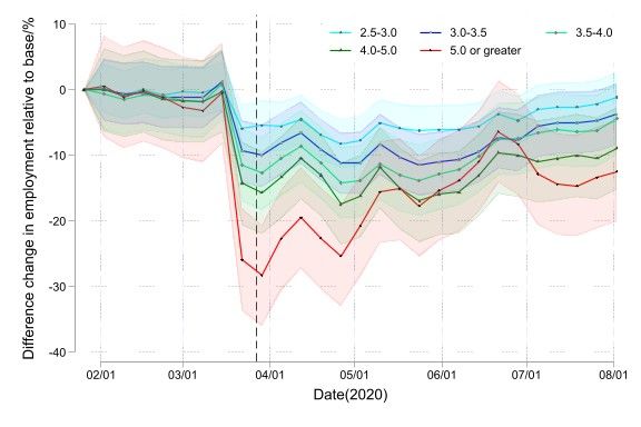
1. Introduction

The economic challenges caused by the 2020 COVID-19 pandemic are almost incalculable. Ever since
the world slid into an unprecedented state of shock-induced paralysis, researchers of all fields have been
trying to analyze the consequences of lockdowns and shutdowns. One economic element of particular
interest has been the labor market. While the level of employment started its drastic decline early
2020, the United States Congress passed a $2.2 trillion relief bill helping those losing their jobs due to
the pandemic by increasing unemployment benefits. This brief’s aim is to analyze the possible effects
on employment of this increase in unemployment insurance (UI). Not only does standard economic
theory suggest that labor supply reacts negatively to a rise in UI, but previous empirical evidence has
documented increases in unemployment durations with more generous UI benefits (see for instance
Atkinson and Micklewright (1991) and Krueger and Meyer (2002)).

The first part of our analysis closely follows the event study conducted by Altonji et al. (2020) and
simply expands the time horizon. They used a linear probability event study model to estimate weekly
employment probabilities of individuals around the time of the CARES Act implementation. Individ-
uals are further grouped by their exposure to the changes in UI benefits. They conclude that groups
of higher exposure do not observe a larger decline in the estimated employment probability, suggest-
ing that the lump-sum increase in UI benefits did not have any instant negative implications for the
labor market. While their analysis is useful, it is limited by the grouping mechanism use of so-called
replacement rate ratios which are inherently correlated with worker’s wages. As noted by the authors,
this identification strategy hence faces the threat of endogeneity and potentially biased estimates. We
address these issues by implementing strategies to reduce the degree of endogeneity. We introduce two
variables controlling for in-group heterogeneity, the first being an hourly wage dummy and the second
a weekly wage dummy.

Overall, we find results similar to Altonji et al. (2020). In particular, there is no notable decline in
the probability of employment related to the CARES Act. However, we want to point out that there
are various reasons to interpret this result with caution. While we are confident about the empirical
approach used in our analysis, there are external factors affecting the interpretation of our results. The
CARES Act had been implemented as a temporary relief. Moreover, the large and sharply negative
effect of the pandemic on the labor market may simply overshadow any potential effects caused by an
increase in UI.

In the second part of the paper, we explore possible labor market effects of public health measures
implemented to slow down the spread of the coronavirus. In particular, we analyze four measures: (1)
stay-at-home orders, (2) closure of non-essential businesses, (3) closure of restaurants and (4) closure
of gyms. These policy measures should serve as evidence for strong negative forces effecting the labor

                                                    2
market, even prior to the CARES Act. All measures largely contribute to a negative trend on the
labor market which complicates the isolation of possible effects due to the CARES Act. And indeed,
with exception of the closure of gyms, we find uniform negative effects of all policy measures on the
probability of employment across all groups. This further demonstrates the strong negative economic
implications from most of these policy measures, and thus the potential of overshadowing the effects
of the enhanced UI benefits.

2. Data

We use micro-data made available by Homebase, a private company which provides timecard data for
small businesses across the United States. In comparison to regular labor market data, this dataset
consists of the exact daily hours worked for every employee in each firm. However, as previously
pointed out by Bartik et al. (2020), the majority of firms in this data are small and rely on hourly
work leaving us with mostly firms in the Food & Drink and Retail sectors. Consequently, it falls short
of providing data on salary workers and firms which do not employ timecards. Hence our conclusions
give insights about small firms operating with hourly workers, while potentially leading to issues with
generalizing our results to the economy as a whole. The dataset ranges from 2018 to present across
all states of the United States. To compute the UI we use the UI calculator by Bachas et al. (2020).
With that, following the methodology by Altonji et al. (2020), we can compute replacement rates after
the implementation of the CARES Act1

                                       UICARES,is   UI2019,is + 600                  600
                    replCARES,is =                =                 = repl2019,is +
                                        w2019,is       w2019,is                     w2019,is

where we define the respective replacement rate as a ratio of UI to average weekly wages. In other
words, it defines the percentage share of a worker’s 2019 wage provided through UI if said worker
becomes unemployed. Here, UI2019,is represents the UI benefit a worker would have been eligible for
in January 2020. This means that if replCARES,is > 1, an individual would be better off receiving UI
benefits. We can further define the replacement rate ratio (RRR) as follows

                                       replCARES,is   UICARES,is       600
                               ris =                =            =1+
                                        repl2019,is    UI2019,is     UI2019,is

which displays the relative change in the replacement rate due to the CARES Act implementation. To
ensure the interpretation ability of our data, we only keep samples with sufficient information. Our
data selection process follows the following steps: First, we only keep the individuals that worked at
least 30 hours per week for each quarter in 2019, and at least 10 weeks per quarter, to make sure our

  1 The   Coronavirus Aid, Relief, and Economic Security Act 2020 promised laid off workers an additional weekly $600

                                                          3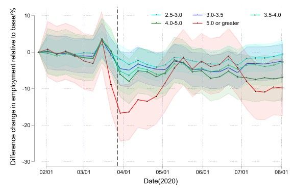
samples have sufficient working time for us to calculate the replacement rate using the UI Calculator.
We also exclude all employees with hourly wages equal to 0, which indicates them as managers or
general managers since they are paid with salaries instead of hourly wages.

Next, only individuals who work for a firm which had been open for more than 40 hours in the base
period are kept in our data to ensure employment before the pandemic. The base period is defined as
the third and fourth week of January 2020. Note that we also substitute the respective state minimum
wage whenever an individual’s wage is below this states required threshold. Table 1 briefly summa-
rizes the data used in our analysis. Our dataset includes 21,033 individuals using the Homebase system.

                          Table 1: Cross-Sector Descriptive Statistics, Base Period

                              Mean       Std. Dev.    Min     25 %         Median     75 %     Max       Observations

           Hours worked       40.17        9.40       8.00    35.02         39.92     44.33    99.66        21,033

           Hourly wage        13.86        4.53       7.25    11.00         13.25     15.87    98.50        21,033

           Weekly wage        543.78      198.35     221.25   419.69       510.70    623.81   3,989.72      21,033

           Pre-CARES                                                                                        21,033
                                  0.51     0.06       0.09     0.50         0.50      0.52     0.65
           replacement rate

           Post-CARES                                                                                       21,033
                                  1.73     0.40       0.27     1.47         1.69      1.96     3.23
           replacement rate

           RRR                    3.40     0.71       1.73     2.91         3.31      3.77      6.56        21,033

3. Empirical Strategy & Results

Next, we briefly introduce the empirical strategy used to estimate the impact of increasing UI benefits
on employment. We implement an event study approach suggested by Altonji et al. (2020)

                              S                                               S X
                                  αs 1{s = t} +          βb 1{b = g} +                    γbs 1{b = g}1{s = t}
                              X                      X                        X
              yigjkt =
                          s=s0                       b                        s=s0    b
                                                                                                                        (1)
                                                                          S
                                                                                 δsigjk 1{s = t}Xigjk + εigjkt
                                                                          X
                                                                      +
                                                                          s=s0

which estimates the probability of employment for each individual i in the respective RRR group g,
industry j, state k as well as time t. We illustrate the allocation of workers to their respective RRR
group and their average hourly wages in Table 2.

                                                              4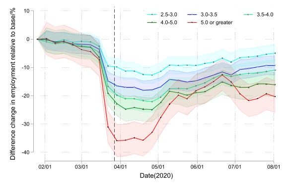
Table 2: Allocation of RRR Groups

                                Variable   Mean    Std. Dev.   Min    25 %    Median   75 %    Max     Observations

             Base Group          RRR       2.31      0.14      1.73   2.24     2.33    2.41    2.49       37,201
                                 Wage      21.41     7.23      7.25   17.00   20.00    24.00   91.00      37,201

             ris ∈ [2.5, 3.0)    RRR       2.78      0.14      2.50   2.65     2.79    2.90    2.99       97,543
                                 Wage      16.23     3.26      7.25   14.00   16.00    18.00   98.50      97,543

             ris ∈ [3.0, 3.5)    RRR       3.25      0.14      3.00   3.15     3.22    3.37    3.49      135,715
                                 Wage      14.07     2.89      7.25   12.35   14.00    15.00   80.00     135,715

             ris ∈ [3.5, 4.0)    RRR       3.70      0.15      3.5    3.56     3.68    3.83    3.99       92,581
                                 Wage      12.25     2.30      7.25   11.00   12.00    13.25   60.00      92,581

             ris ∈ [4.0, 5.0)    RRR       4.37      0.27      4.00   4.14     4.32    4.57    4.99       59.732
                                 Wage      9.87      1.64      7.25   9.00    10.00    12.00   60.00      59,732

             ris ≥ 5             RRR       5.40      0.29      5.00   5.15     5.36    5.60    6.56       14,201
                                 Wage      7.90      1.14      7.25   7.25     7.46    8.25    20.00      14,201

Here, the indicator function 1{s = t} defines a set of week dummies, 1{b = g} defines the respective
affiliation of an individual in g. The reference group contains workers who have a RRR less than
2.5 and the base period are the two weeks from January 19 to Febuary 1. The control vector Xigjk
contains the pre-CARES replacement rate, baseline wage and industry (Panel (a)). Additionally, we
define a second set of controls consisting of the controls mentioned above as well as a set of time-
varying controls for weekly COVID-19 cases per capita and an indicator for active policy measures in
a particular state (Panel (b)).2

3.1. Event Study
The Figures 1(a) and 1(b) show the effect of RRR on the probability of employment relative to the
reference group in the base period following Altonji et al. (2020). We plot γgt in (1), i.e. the inter-
action of week indicators t and the RRR groups g, over time. These coefficients then determine if an
individual i was employed at time t. The dotted line represents the week in which the CARES Act was
signed into law. Figure 1(a) shows that following the week of March 22, which is immediately before
CARES, there is no variation in the declines of employment probabilities across different RRR groups.
Note that while those groups differ regarding the increase of received UI benefits, they seem to have
similar trends. We observe that the group with RRR of 5 or above, which consists of individuals who
supposedly benefit the most from the increase in UI, was the earliest to start showing an upward trend
in employment probability. Also note that following the sharpest decline of all the groups, this group

   2 Indicators include stay-at-home orders, mandatory closure of non-essential businesses, mandatory closure of restau-

rants and mandatory closure of gyms

                                                                 5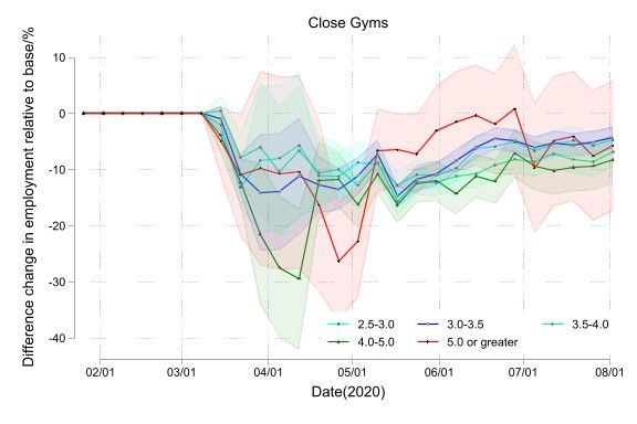
seems to have the steepest incline, especially in the reopening phase from Mid-June to the first week
of July. Furthermore, it seems that there is a significant drop in the first week of July for all groups.
This is very likely to result from the 4th of July holiday.

           Figure 1(a) & 1(b): Uncontrolled Coefficients of RRR on Probability of Employment

In Figure 1(b) we control for state restrictions and the number of new COVID-19 cases in each state
per week. The results seem to be similar to those from panel (a), but with slightly higher rates for
some periods. The trend is equivalent to panel (a) and it seems that the increase in UI does not affect
labor force on the extensive margin. This is in line with the finding of Altonji et al. (2020).

As we observe significant heterogeneity, even within groups, we conduct a controlled regression analysis
where we use hourly wages or weekly wages of 2019 as additional variables respectively3 . Ideally, we
want no variation across groups in the outcome of interest prior to the introduction of CARES. As
wages are expected to be a main driver for this heterogeneity (see the standard deviations in Table 2),
we employed the previously stated controls. The base regression, however, is still based on equation
(1), hence our regression equation can then be expressed as follows

                              S                                           S X
                                     αs 1{s = t} +        βb 1{b = g} +               γbs 1{b = g}1{s = t}
                              X                      X                    X
                   yigjkt =
                              s=s0                    b                   s=s0    b
                                                                                                             (2)
                                      S                               S
                                             θsigjk 1{s = t}wigjk +          δsigjk 1{s = t}Xigjk + εigjkt
                                      X                               X
                                 +
                                      s=s0                            s=s0

where w defines the respective wage measure strategy.

  3 note   that these additional controls correspond to two different identification strategies

                                                               6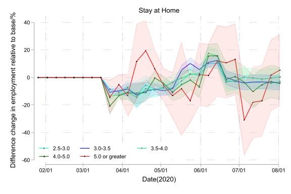
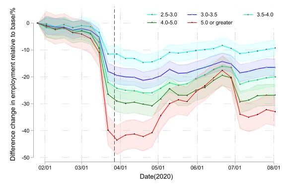
First, we focus on the strategy adding hourly wages as a control to our regression analysis. Reflect-
ing upon Figure 2(a), corresponding to Panel (a), we see that for workers with different RRR, the
overall trends of changes of probability of being employed relative to the reference group were the
same. Starting in week of March 22 after multiple states began to lock down their economies, the
employment probabilities all dropped significantly. Among these changes, workers with RRR of 5 or
above suffered the most, with a more than 35 percentage point drop in probability. Starting in week
of April 19, however, probabilities began to increase. For workers with RRR below 5, probabilities
began to stabilize in week of May 3. For workers in the highest RRR group, the probability of being
employed relative to the reference group did not stabilize until week of July 5. After this week, the
probabilities of all groups were increasing modestly.

                  Figure 2(a) & 2(b): Coefficients of RRR with hourly wage control

Figure 2(b) shows that the overall trends of changes of probability of being employed relative to the
reference group were the same. Starting in week of March 22 after multiple states began to lock down
their economies, the employment probabilities all dropped significantly. Among these changes, workers
with 5 or higher RRR again seem to suffered the most, with a more than 40 percentage point drop in
probability. We observe a flattening of all trends across RRR groups at the time the CARES Act was
implemented, indicating no significant effect of the increase in UI benefits on the probability of being
employed. Starting in week of April 19, however, the probabilities began increasing. For workers with
RRR below 5, probabilities began to stabilize two weeks later.

We can see that for Panel (a), employing the additional wage control has minor effects of the overall
results. However, note that we estimate a much smoother process when using the full set of available
policy controls in Panel (b). This further suggests potentially biased results with the initial identifica-
tion strategy as used by Altonji et al. (2020). From these two graphs, it is evident that when we control
for hourly wages, the probability of getting unemployed is highest for people with a RRR within 2.5-3

                                                    7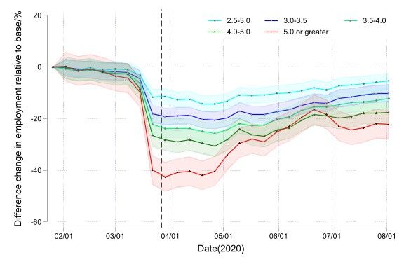
and lowest for people with with the largest ratios.

In Figures 1(a), 1(b), 2(a) and 2(b), we found two waves of unemployment for group 5, the group of
people with RRR above 5. The first tiny wave appears between calendar week 21 and 23, with a locally
lowest point in the week of May 24. Another wave begins from the week of June 28, and reaches its
lowest point two weeks after that. Between the two waves, the line of group 5 intersects that of group
4 twice, exceeding the line of group 4 for 5 weeks. It implies that there is a temporary period during
which the expansion of UI has less negative effect on the workers with replacement rate ratio above 5
than those with replacement rate ratio between 4.0-5.0. During March 24 and July 12, group 5 shows
drastic fluctuation. We have two possible explanations for the fluctuations, one is that group 5 has
substantially fewer data points than other groups, hence the estimation result is more volatile.

                    Figure 3(a) & 3(b): Coefficients of RRR with weekly wage control

Compared to group 4, which has about 3,000 observations, group 5 have only about 720 observations.
Another reason is that UI does have larger impact on the unemployment of workers with high replace-
ment rate ratio. This impact is not obvious initially because of the large shock of pandemic, but it
matters later on.

Next, we plot γgt from regression equation (2) where w represents weekly wages. For Figure 3(b) we
find similar results and again relatively flat trends around the time CARES was implemented. First
we observe an increase interrupted by a sudden drop around mid-March. The sharp decline is followed
by a relatively stable trend indicating a slow recovery. The drop can obviously be explained by the
COVID-19 outbreak all over the US, whereas the early increase can be deduced from higher earnings
relative to the base period before the crisis hit.

For cross-group comparison, we observe larger negative effects with higher RRR. Also, note that the

                                                      8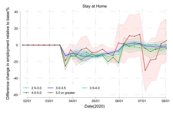
main difference between Panel (a) and Panel (b) is that the latter has smaller coefficients, larger drops
for each group larger between group differences.

3.2. Policy Effects
Furthermore, we analyze the direct effects of policy measures intended to restrict the spread of COVID-
19 on employment in the respective RRR groups.4 Ideally, we here want to capture and isolate the
potential negative effects of various measures that have been set it place across the United States. For
this part, our empirical strategy can be presented as follows

                                S                                          S X
                                      αs 1{s = t} +       βb 1{b = g} +                γbs 1{b = g}1{s = t}
                                X                     X                    X
                  yigjkt =
                               s=s0                   b                    s=s0    b
                                                                                                              (3)
                        S                                 4 X
                                                            S X
                               δsigjk 1{s = t}Xigjk +                          1{b = g}1{s = t}q + εigjkt
                        X                                 X
                                                                          h                      h
                    +                                                    ηbs
                        s=s0                              h=1 s=s0   b

where we define q h as an indicator of whether a policy measure is in place or not, i.e.

                                                q h = 1{policy h in place}

Additionally, we run single policy regressions to further examine the effects of these political measures
on the the labor market.5 The corresponding regression can be defined as follows

                                S                                          S X
                                      αs 1{s = t} +       βb 1{b = g} +                γbs 1{b = g}1{s = t}
                                X                     X                    X
                  yigjkt =
                               s=s0                   b                    s=s0    b
                                                                                                              (4)
                               S                              S X
                                    δsigjk 1{s = t}Xigjk +                   1{b = g}1{s = t}qh + εigjkt
                               X                              X
                                                                          h
                         +                                               ζbs
                             s=s0                             s=s0   b

Note that due to large outliers as well as small sample size the group with a RRR of 5 and above
should be interpreted with caution.

As of the week of March 15, several states started to place a stay- at-home order for non-essential
                                                    h       h
workers (among others). The following graphs plots ηgt and ζgt over time for the respective group,
where h in this case represents the ”stay-at-home” orders. Figure 4† indicates that from March 15
to May 10, all groups with RRR lower than 5 suffer negative effects on employment. Specifically,
before week the week of April 19, individuals with the highest RRR faced a substantial increase in the

  4 Note   that graphs with † are related to this strategy.
  5 Consequently,   graphs marked with ‡ are related to this strategy

                                                               9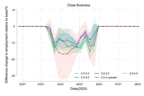
probability of employment while other groups saw decreasing rates.

           Figure 4† & 4‡ : Effects of Stay-at-Home Orders on Probability of Employment

After a brief upward trend, indicating a decrease in the effect of the policy, we observe another phase of
decline in the week of June 21, followed by a rather stabilized trend around zero. Hence, as expected,
the ”stay-at-home” orders seem to have a negative effect on employment throughout all groups. Figure
4‡ again indicates that from the week of March 15 to the end of March, all groups were negatively
affected by the stay-at-home policy. As of the week of June 7, the effect of the stay-at-home policy
decreased, and groups with the highest RRR were positively affected by the policy and had a rapid
increase in employment probabilities than other groups. The second lowest RRR group had the lowest
unemployment rates through most part of the period. From June 28 to July 19 the the group with
the lowest RRR replaced them after seeing a sharp decline in employment probabilities to about 30
percentage points. In general, we observe that groups which are affected more by the increase in UI
benefits suffered more from the stay-at-home orders than those with lower RRR.

Next, we focus on ordered non-essential businesses closures. With the stay-at-home order in place,
more and more states extended their list of policies aiming to contain the spread of COVID-19. One
common measure is the mandatory closure of non-essential businesses, which had expected significant
effects on employment. Figure 5† and Figure 5‡ present these effects for the respective RRR groups.
First, Figure 5† which shows that all employees in the groups was negatively effected by the policy,
and the lowest replacement ratio group shows more volatility in the unemployment effect especially
for the first and last weeks where the policy was in place.

                                                   10
Figure 5† & 5‡ : Effects of Closure of Non-essential Businesses on Probability of Employment
We then have figure 5‡ which does a good job in capturing and depicting these massive negative im-
pacts on the probability of being employed with reaching -15 percentage points. Although, one might
expect larger negative effects for those with larger marginal returns to an increase in UI benefits, our
results offer a different conclusion. It seems that there are no significant differences in severity between
groups. Also, note that in both figures there is a strong upward trend before the effect seems to vanish,
suggesting that the majority of these business closures were rather short-lived.
Additionally to non-essential business closures, we analyzed the effects of restaurant closures. This is
mainly motivated by the composition of our data, as roughly half of the individuals in our sample work
in the Food & Drink sector. The graphs below indicate a drop around the time the measure was put
into place followed by a relatively flat trend. The drop was an overall for the group, but it seems that
there was increase especially for the first period for the three lowest replacement ratio groups. After
that, all group’s employment probabilities decreased substantially by about less than 50 percentage
points through the period the policy implemented. The second to the lowest replacement ratio seems
the most negatively affected by this policy, while the lowest group was the least affected. The upward
trend towards the end of our panel seems to reflect a higher employment among those restaurants
which are open, relative to the base period.
11Figure 6† & 6‡ : Effects of Restaurant Closures on Probability of Employment
Lastly, we analyze the final policy control, namely gym closures across states. Figure 7† and Figure
7‡ present the effect of closing gyms on employment. Starting with the week of March 8, some states
mandated to close gyms for customers. Figure 7† shows that around the week of April 19, all groups
seem to have a negative response to the gym closures. From the Mid-May onwards, these negative im-
pacts increased further. Figure 7‡ indicates immediate responses in week 11 as all groups face negative
impacts on employment from the close-gyms policy. In general, both figures show that gym closures
have had an increased negative impact on all groups’ employment, and it continues to have that.
From all the policies that are examined here, Stay at home order and gym policy closures policies had
the largest effects on employment reaching up to -30 percentage points. Followed by close restaurant
policy, where the employment probabilities decreased more than 25 percentage points, and non-essential
business closure which had the lowest affect among all policies, where the employment falls 15 percent-
age points. While we have a short term affect by the non-essential business closure on employment,
gym closure seems to have long term effect on employment among all the policies.
12Figure 7† & 7‡ : Effects of Gym Closure on Probability of Employment
Finally, we observe uniform negative effects of all these measures on all RRR groups prior to the
enactment of the CARES Act. We therefore can empirically show that there were large negative labor
markets persistent in advance to the lump-sum increase in UI, which might lead to the relatively
insignificant results in the first part of this analysis as these strong negative tendencies are expected
to at least partially overshadow any potential effect of a change in UI.
4. Conclusion
In this report, we analyzed the impact that enhanced UI benefits had on the probability of employ-
ment during the COVID-19 pandemic. We found no evidence that the enhanced benefits influenced
tge employment probability, and most replacement rate ratio groups had employment trends compared
to the base period. We also found that individuals who would benefit the most from UI (higher RRR)
faced lower unemployment rates compared to others. Additionally, this group re-entered the labor
market faster than other groups, especially during the reopening period. These results are similar
to our findings when incorporating the weekly and hourly wage controls. Lastly, we examined the
effect of COVID-19 policies implemented in various states to measure their effect on the labor market.
The observed policies generally decreased employment probabilities significantly. Moreover, we find
significant negative effects of these measures on the probability of employment prior to the CARES
Act implementation. Along with the limited duration of the enhanced UI benefits and the difficulty
of turning down a job in pandemic, our results suggest that many of these negative labor market dy-
namics preceding the increase in UI may have been overshadowing the possible effects of the CARES
Act.
Our results support the findings by Altonji et al. (2020), showing that during this period, higher
unemployment insurance benefits did not lead to lower employment probabilities. In addition to the
overshadowing effect of the pandemic itself, there are several other hypotheses for why the UI effects
13seem to be marginal. For instance, Boar and Mongey (2020) provide a dynamic model which contains
other possible causes for employees to return to their previous job even when received UI benefits
exceed the wages at the previous job. The temporary nature of CARES Act, the uncertainty that the
return-to-work offer will hold, the difficulty for searching for a new job and the prospect of a perma-
nent lower wages caused by unemployment during recession are mentioned as reasons. Moreover, their
empirical results show that workers would be unlikely to reject a return-to-work offer at the same wage.
Similar results have been found by Finamor and Scott (2020). They also conclude that UI expansions
did not increase layoffs during the pandemic or provide a disincentive for workers to returning to their
jobs over time, and that these findings are uniform across all groups. Finally, a study by Ganong
et al. (2021) exploring the effects of increasing UI on job searches during the pandemic found stable
job-finding dynamics. This can be interpreted as further explanation for a rather insignificant effect
of the CARES Act on employment probabilities.
In conclusion, large overshadowing negative labor market dynamics caused by various policy measures
in place to slow down the spread of COVID-19, the temporary nature of the UI expansion, as well as
solid empirical evidence for stable job-finding dynamics, are all possible explanations for the insignifi-
cant implications of enhanced unemployment benefits on employment, as we found. Importantly, our
results do not necessarily imply that enhanced benefits would continue to have minimal impact later
in the pandemic as the economic recovery continues.
5. Bibliography
Altonji, J., Contractor, Z., Finamor, L., Haygood, R., Lindenlaub, I., Meghir, C., ODea, C., Scott, D.,
Wang, L., Washington, E., 2020. Employment effects of unemployment insurance generosity during
the pandemic. Yale University Manuscript.
Atkinson, A. B., Micklewright, J., 1991. Unemployment compensation and labor market transitions:
a critical review. Journal of economic literature 29 (4), 1679–1727.
Bachas, N., Ganong, P., Noel, P., Vavra, J., Wong, A., Farrell, D., Greig, F., 2020. Initial impacts
of the pandemic on consumer behavior: Evidence from linked income, spending, and savings data.
NBER Working Paper (w27617).
Bartik, A. W., Bertrand, M., Lin, F., Rothstein, J., Unrath, M., 2020. Measuring the labor market at
the onset of the covid-19 crisis. Tech. rep., National Bureau of Economic Research.
Boar, C., Mongey, S., 2020. Dynamic trade-offs and labor supply under the cares act. Becker Friedman
Institute at The University of Chicago, 16.
14Finamor, L., Scott, D., 2020. Employment effects of unemployment insurance generosity during the
pandemic. Munich Personal RePEc Archive:MRPA Paper (102390).
Ganong, P., Greig, F., Liebeskind, M., Noel, P., Sullivan, D., Vavra, J., 2021. Spending and job search
impacts of expanded unemployment benefits: Evidence from administrative micro data. University
of Chicago, Becker Friedman Institute for Economics Working Paper (2021-19).
Krueger, A. B., Meyer, B. D., 2002. Labor supply effects of social insurance. Handbook of public
economics 4, 2327–2392.
15You can also read