The population doctrine in cognitive neuroscience - arXiv

The population doctrine in cognitive neuroscience

                        R. Becket Ebitz1* and Benjamin Y. Hayden2

1
 Department of Neuroscience
Faculty of Medicine
Université de Montréal
Montréal, QC Canada
2
Department of Neuroscience,
Center for Magnetic Resonance Research, and
Center for Neuroengineering
University of Minnesota
Minneapolis, MN USA

*Corresponding author:
      R. Becket Ebitz
      Department of Neuroscience
      Faculty of Medicine
      Université de Montréal
      Montréal, QC Canada
      Email address: becket@ebitzlab.com

                                                                    1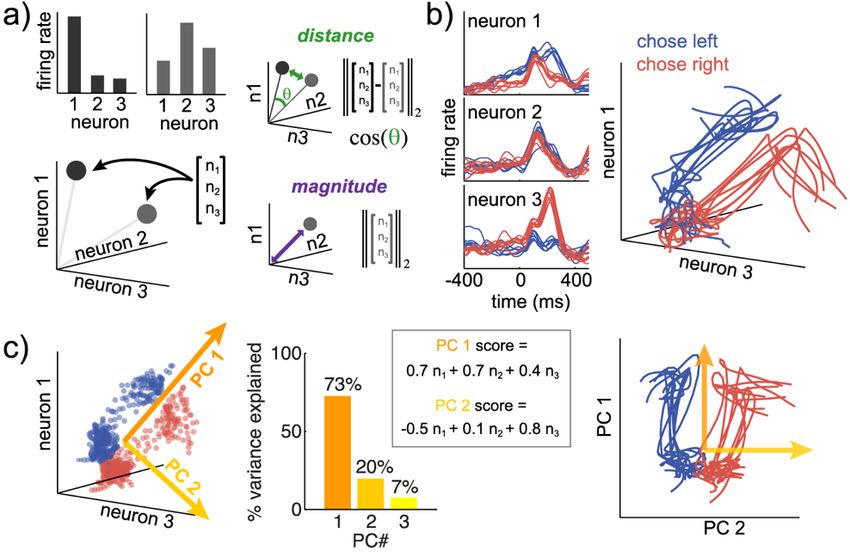

SUMMARY
       A major shift is happening within neurophysiology: a population doctrine is drawing
level with the single-neuron doctrine that has long dominated the field. Population-level ideas
have so far had their greatest impact in motor neuroscience, but they hold great promise for
resolving open questions in cognition as well. Here, we codify the population doctrine and
survey recent work that leverages this view to specifically probe cognition. Our discussion is
organized around five core concepts that provide a foundation for population-level thinking: (1)
state spaces, (2) manifolds, (3) coding dimensions, (4) subspaces, and (5) dynamics. The work
we review illustrates the progress and promise that population-level thinking holds for cognitive
neuroscience—for delivering new insight into attention, working memory, decision-making,
executive function, learning, and reward processing.

                                           IN BRIEF
       The population doctrine holds that the fundamental computational unit of the brain is the
population. This view holds great promise for resolving open questions in cognition. We discuss
five core concepts of population analysis and review relevant papers.

                                                                                                    2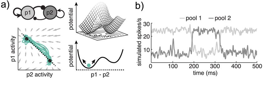

INTRODUCTION
       Cognition gives us the flexibility to selectively attend to a stimulus, hold information in
mind, pursue arbitrary goals, implement executive control, or decide between actions by learning
about and weighing beliefs about their outcomes. Neurophysiology has revealed much about the
neural basis of cognition over the last fifty years, generally by examining responses in one
neuron at a time. However, brain areas contain hundreds of millions of neurons (Herculano-
Houzel 2009) and somewhere between the scale of single neurons and the gross pooling in EEG
or fMRI, neuronal populations produce macroscale phenomena that are poised to link the scale
of single neurons to the scale of behavior.
       The term population doctrine describes the belief that the population, not the neuron, is
the fundamental unit of computation (Saxena and Cunningham 2019). This idea is not new: some
researchers have always studied how neurons behave collectively, whether that was Hebb’s cell
assemblies in the 1940’s (Hebb 1949) or Georgopolous’ population vectors in the 1980s
(Georgopoulos, Schwartz, and Kettner 1986). Population ideas have always been influential in
theoretical neuroscience, but they have sometimes lain dormant among experimentalists.
However, with the development and spread of new technologies for recording from large groups
of neurons, we have seen a resurgent interest in population-level thinking. Alongside new
hardware, an explosion of new concepts and analyses have come to define the modern,
population-level approach to neurophysiology (Yuste 2015; Saxena and Cunningham 2019;
Jazayeri and Afraz 2017; Shenoy and Kao 2021; Vyas et al. 2020). Although advances in high-
yield neural recordings were critical for the resurgence of these ideas, high-yield recordings are
neither necessary nor sufficient nor sufficient to make a population neurophysiology paper.
Instead, what defines the field is its object: the neural population. To a population
neurophysiologist, neural recordings are not random samples of isolated units, but instead low-
dimensional projections of the entire manifold of neural activity (Gallego et al. 2017; Jazayeri
and Afraz 2017). Here, we will explain this and other fundamental ideas in population
neurophysiology, while illustrating why we believe this approach holds such promise for
advancing our understanding of cognition.

                                                                                                     3

THE STATE SPACE
        For a single-unit neurophysiologist, the canonical analysis is a neuron’s peristimulus time
histogram (PSTH). For a population neurophysiologist, it is a neural population’s state space
diagram (Figure 1A). Instead of plotting the firing rate of one neuron against time, the state
space diagram plots the activity of each neuron against one or more other neurons. At every
moment in time, the population is at some neural state: it occupies some point in neuron-
dimensional space, or, identically, produces some vector of firing rates across recorded neurons.
Time is a function that links neural states together; it turns sequences of neural states (or sets of
PSTHs) into trajectories through the state space (Figure 1B). (Trajectories have interesting
implications for thinking about how the brain computes. We will return to them in Dynamics.)
Especially in cognitive studies, neural states may be called representations: a somewhat
contentious term meant to highlight the correspondence between a neural state and some percept,
memoranda, computation, or behavior (see Text Box: Representations?).
        Re-casting population activity as a neural state can suggest new hypotheses. As vectors in
neuron-dimensional space, neural states both point in some direction, and have some magnitude
(Figure 1A). Because the direction of a neural state vector is related to the pattern of activity
across neurons, it is probably unsurprising that state vector direction encodes object identity in
the inferotemporal cortex (IT) (Jaegle, Mehrpour, and Rust 2019; Chang and Tsao 2017).
However, it is maybe more surprising that this second feature—neural state magnitude—also
matters: it predicts how well objects will be remembered later (Jaegle, Mehrpour, and Rust 2019;
Jaegle et al. 2019). When we pause to realize that magnitude is essentially a sum of activity
across neurons, this may seem like an obvious analysis, or one that just recapitulates the cell-
averaged PSTH. However, this is a sum across all neurons—regardless of their tuning
properties—and it is taken without normalization. For a single-neuron neurophysiologist, it is
essential to normalize the dynamic range of neurons before averaging—this is the only way to
produce a clear picture of the response profile of an “average” neuron. However, for a population
neurophysiologist, more concerned with the holistic population than the average neuron,
differences in the dynamic range between neurons are a critical part of the signal. Because spikes
are energetically costly and large-magnitude neural states require more spikes, understanding this
aspect of the population code could be particularly interesting in cognitive domains where
energetic efficiency is a concern, like in classic, energetically costly conflict signals (Ebitz et al.

                                                                                                          4

2020; Ebitz and Platt 2015) or in understanding why we follow simple rules in lieu of less
efficient, but more flexible decision-making processes (Cohen et al. 2021; Ebitz et al. 2020).
       Because the state space gives us a spatial view of neural activity, it makes it natural to
start to think about spatial relationships between different neural states, to reason about distances
(Figure 1A). There are many ways to measure the distance between neural states, including the
Euclidean distance, the angle between state space vectors (which decorrelates distance from any
differences in magnitude) and the Mahalanobis distance (which accounts for the covariance
structure between neurons). (See Walther et al., 2016, for discussion of distance measures in
neural data analysis.) Distance measures have many applications, including for reasoning about
how neural states evolve over time. For example, in a slowly changing environment, we might
expect neural states to also change slowly over time. However, there can be sudden jumps in
neural states across pairs of trials (Karlsson et al. 2012; Durstewitz et al. 2010; Bartolo et al.
2020; Russo et al. 2021; Ebitz et al. 2018; Malagon-Vina et al. 2018). These jumps could reflect
cognitive or behavioral discontinuities—sudden changes in our beliefs or policies—and are thus
difficult to reconcile with simple cognitive models of sequential decision-making, where
information is integrated slowly across multiple trials and behavior changes gradually, rather
than suddenly (Bartolo and Averbeck 2020). Instead, jumps may better resonate with
hierarchically structured models, where inferences are being made at the level of policies, rather
than actions (Collins and Koechlin 2012; Eckstein and Collins 2020).
       Measures of distance can also be combined with clustering algorithms from machine
learning to examine the similarity between neural responses across task conditions (Kriegeskorte
et al. 2008; Hunt et al. 2018), characterize hierarchical relationships between different pieces of
information (Kiani et al. 2007; Reber et al. 2019), or examine the variance within or between
task conditions—a factor that changes with learning (Thorn et al. 2010) and across goal or belief
states (Ebitz et al. 2018). Perhaps the most systematized approach for reasoning about spatial
relationships between neural states is Representational Similarity Analysis (RSA), a method first
developed in neuroimaging that has been extensively reviewed in that context (Kriegeskorte et
al. 2008; Diedrichsen and Kriegeskorte 2017). In neurophysiology, RSA has been used to ask
how semantic knowledge shapes mnemonic representations (Reber et al. 2019), to compare the
computations involved in decision-making across regions (Hunt et al. 2018), to characterize the
stability of representational structure over working memory (Spaak et al. 2017), to examine how

                                                                                                      5

rules shape information processing across regions (Ebitz et al. 2020), and to contrast the
contributions of different structures to encoding task dimensions (Keene et al. 2016). In fMRI,
RSA is often interpreted as a kind of neural recapitulation of perceptual or psychological
similarity. However, because we still lack whole-brain resolution, neurophysiologists should be
cautious about these kinds of interpretations because different representational structures may be
found in different brain regions (Hunt et al. 2018; Keene et al. 2016).
       Neural state space diagrams can have as many axes as there are recorded neurons.
However, neural activity often only varies along a smaller number of directions in the state
space, known as dimensions (Gao and Ganguli 2015; Gao et al. 2017; Low et al. 2018; Gallego
et al. 2018; 2017; Chaudhuri et al. 2019; Lehky et al. 2014). Because activities of different
neurons are correlated with each other (Cohen and Kohn 2011), every neuron does not make an
independent contribution to the population (Umakantha et al. 2020). It is generally a combination
of neurons that drive most of the variability in neural activity. We take advantage of this
redundancy by using dimensionality reduction to compress neuron-dimensional state spaces onto
a smaller number of axes (Cunningham and Yu 2014). There are many ways to choose these
axes, including principal components analysis (PCA; Figure 1C). Other dimensionality
reduction methods, developed specifically for neurophysiology data, can take advantage of the
temporal structure of this data and even solve other problems, like combining together
(“stitching”) non-simultaneously recorded data sets (Yu et al. 2009; Pandarinath et al. 2018;
Kobak et al. 2016; Williams et al. 2018). Because it is hard for humans to reason about higher
dimensional spaces, dimensionality reduction is helpful for exploratory analyses, but it can also
be an important part of data processing pipelines when we want to focus on only the important
dimensions in neural activity.
       Is there always a one-to-one correspondence between a neural state and a particular
cognitive state? There is some evidence that multiple patterns of activity could implement the
same function at different moments in time (Malagon-Vina et al. 2018; Rule et al. 2020; Driscoll
et al. 2017; Ebitz et al. 2018). This idea is known as multiple realizability in philosophy of mind.
For example, in uncertain environments, decision-makers often pass through some period of
exploration in between longer periods of following some rule or policy (Wilson et al. 2021; Ebitz
et al. 2018 and 2019). Exploration produces the kinds of sudden jumps in neural activity we
introduced with the concept of distances, but it also disrupts long-term autocorrelations between

                                                                                                    6

neural states and promotes new learning. The pattern of activity that implements a policy after
exploration is not the same as the pattern that existed before, even when subjects are just
returning to an old policy. The ability to implement the same policy via slightly different neural
states could offer some benefits in nonstationary environments (Ajemian et al. 2013; Chambers
and Rumpel 2017), but it also implies that the neural state spaces may have many sloppy
dimensions—dimensions along which neural activity can vary without affecting cognition and
behavior—and a smaller number of stiff dimensions in which comparatively small differences
between neural states can have big implications for cognition and behavior. We will return to
these concepts when we discuss Coding Dimensions and Subspaces.

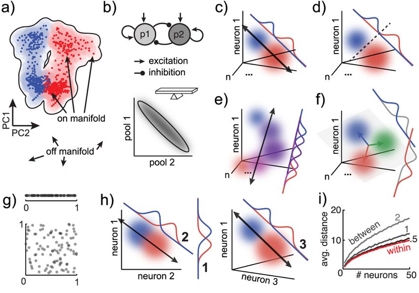
Figure 1: Neural state spaces and dimensionality reduction
A) A neural state is a pattern of activity across a population of neurons. Neural states can be
represented as histograms of firing rates across neurons (top left) or as points or vectors in
neuron-dimensional state space (bottom left). The state space representation makes it more
natural to think about neural activity geometrically. We can use this as a starting point for
reasoning about the distance between different neural states (top right), whether distance is
measured via the Euclidean distance, cosine angle, or some other measure. It also illustrates the
geometric interpretation of state magnitude (bottom right), which is the neural state’s distance
from the origin, the length of the neural state vector.
B) Peri-stimulus time histograms (PSTHs) plot the average firing rate of single neurons as a
function of time, aligned to some event. Spikes are discrete and noisy, so we smooth spike trains

                                                                                                     7

by averaging across trials or by smoothing spikes in time. Both were done here to data from
(Ebitz et al. 2018) (10-trial averages, gaussian smoothing, σ = 25 ms). We can plot these traces
in neural state space, in which case they are called neural trajectories: paths linking neural states
over time.
C) To reduce noise or compress neuron-dimensional state spaces for intuition or visualization,
we use dimensionality reduction methods like principal components analysis (PCA). PCA finds
an ordered set of orthogonal (independent) directions in neural space that explain decreasing
amounts of variability in the set of neural states. The first principal component (PC 1) is the
direction vector (linear combination of neuronal firing rates) that explains the most variance in
neural states (here, 73%). It is often related to time. PC 2 is the direction vector that explains the
next most variability, subject to the constraint that it is orthogonal to PC 1, and so on. Right)
Projecting neural activity onto a subset of the PCs (here, the first 2) flattens our original 3-
dimensional example into a 2-dimensional view that still explains 93% of the variability in
neural states.

                               Text Box 1: REPRESENTATIONS?
       Representation is the process by which one instantiation of some phenomena is replicated
in another form (Kosuth, 1965; Churchland and Sejnowski 1990; Brette 2019). An apple can be
represented in a painting or in a pattern of activity across a group of neurons. It seems almost
trivial to use the word “representation” to refer to the neural correlate of a stimulus, memoranda,
cognitive process, or action, yet the word is contentious. Why?
       For motor neurophysiologists, the term “representation” is loaded, in part, by the
historical influence of sensory coding frameworks in this domain. Rather than inverting the
sensory-coding model to focus on how neural activity produces movement, it can be tempting to
look for “representations’' of movement parameters (Vyas et al. 2020; Fetz 1992; Michaels,
Dann, and Scherberger 2016). However, while a representation of sensory information may give
us some insight into the processes that shaped it—some features may be emphasized, others
eliminated, for example—finding a neural representation of movement velocity cannot tell us
how high velocity movements will be generated (Cisek 2006).
       We have introduced representations as pictorial phenomena—as an image of some neural
process—but the term representation can also have mechanistic connotations. We tend to think
of representations as acting, much like a symbol, to hold information, manipulate it, or pass it
between regions (Barack and Krakauer 2021), but this use of the term should always be met with
two questions: 1) who is interpreting these symbols and 2) how are they doing so?

                                                                                                     8

This mechanistic representationalism is likely inherited from cognitive science, a field
where mental representations are mechanisms for thought: structures on which computations act.
However, despite the similarity in language, a neural representation is not the same thing as a
mental representation and the former is not evidence for the latter (Baker et al. 2021; Barack and
Krakauer 2021). Consider value-based decision-making. Many regions represent value, in the
sense that we can decode value information from them (Vickery, Chun, and Lee 2011; Hunt and
Hayden, 2017). We could conclude that these regions function to represent value for other
regions to act on. However, value representations do not need to have representational functions.
It is just as probable that they are a byproduct of the computations needed to execute choices,
which happen to be related to the quantity we calculate as value (Hayden and Niv 2021; Fine and
Hayden, 2021).
        Avoiding the term “representation” leaves us using convoluted language to describe
patterns of neural activity that correspond to some event. It is not incorrect, in our view, to say
that part of a neural state space represents a task demand or that a neural trajectory represents a
sensorimotor transformation, provided we remember that representation is not necessarily the
function of that pattern of activity.

                                        THE MANIFOLD
        Because activity of neurons tends to be correlated with each other, because the wiring
between neurons constrains what patterns of neural activity are possible, neural states often only
vary along a small number of dimensions in the neural subspace. To put it another way, there is a
lot of white space in our state space diagrams: neural activity tends to occupy fewer neural states
than it would if each neuron made an independent, random contribution to population activity.
The part of the neural state space that contains the states that we observe is called the neural
manifold (Figure 2A).
        We have at least two notions of a manifold. The first—the one we referred to when we
said that neural recordings are a low-dimensional projection of an entire manifold of neural
activity (Gallego et al. 2017)—might be better called the “Manifold”: this is the space that
encompasses all the states that are possible, the states we would observe if we could record
forever, from all the neurons. However, another common usage refers to the space containing on-

                                                                                                      9

task neural states recorded from a small number of neurons during a finite number of trials. This
subtle distinction is why there is no guarantee that a manifold will be the same across tasks,
states, or long periods of time. In practice, they often are (Gallego et al. 2018; 2020; Chaudhuri
et al. 2019), though it may be possible to learn to generate “new” neural states, given sufficient
time and experience (Oby et al. 2019). The difference between the manifold and the Manifold is
also why it is meaningful to say that it is easier to learn to generate neural states that are on the
manifold than states that are in the white space (Sadtler et al. 2014; Oby et al. 2019): off-
manifold neural states may not be impossible, so much as rare. (Of course, “manifold” is also
just a generic mathematical term, so it occasionally appears in other contexts, like to refer to the
space containing the neural states that encode some piece of information (Sohn et al. 2019;
Okazawa et al. 2021). We will return to this in Coding Dimensions.)
       Because manifolds are spaces, they have geometric properties, including a
dimensionality—meaning the number of dimensions that are needed to describe them. Different
dimensionalities might be better for different computations (Figure 2B). Theoretical work
suggests that the dimensionality of neural activity could be yoked to the dimensionality of the
task (Gao et al. 2017; Gao and Ganguli 2015). Though it is a bit harder to think about tasks
geometrically, they can, like manifolds, have an intrinsic dimensionality. If we choose to move
left or right based on a single piece of information (like the direction of moving dots), we only
need a 1-dimensional manifold to represent the evidence for left-or-right. If it matters that we
decide at a particular time, we may need a second dimension to keep track of time, but the
critical point is that laboratory tasks are often low-dimensional.
       Although the number of dimensions is generally obvious in motor tasks, this is not
always true of cognitive tasks (Akrami et al. 2018; Chen et al. 2020; Constantinople et al. 2019;
Filipowicz et al. 2020; Glaze et al. 2018). For example, mice, when given an essentially 1-
dimensional cognitive task (choosing between 2 images), made decisions that depended on
completely irrelevant information (like image locations, past rewards, and past choices (Chen et
al. 2020)). Behavior had many more dimensions than the task. This is neither specific to that task
(Akrami et al. 2018; Constantinople et al. 2019) nor some artifact of the difficulty of designing
good tasks for rodents. Humans also consistently overestimate the dimensionality of cognitive
tasks (Glaze et al. 2018; Filipowicz et al. 2020). We would argue that the brain is generally also
engaged in task-irrelevant processing, and any extra-task information would also increase

                                                                                                        10

manifold dimensionality beyond the dimensionality of the task. Throughout the brain, we find
signals that fluctuate with arousal (Ebitz and Platt 2015; Vinck et al. 2015; Engel et al. 2016;
Engel and Steinmetz 2019) or irrelevant movements (Musall et al. 2019; Vinck et al. 2015).
Indeed, there is some empirical evidence that manifolds can be higher dimensional than the task
(Low et al. 2018), though more work is needed to understand how the dimensionality of neural
manifolds is related to the dimensionality of tasks and/or behavior.
       Some theoretical work suggests that there may be computational benefits to higher
dimensional manifolds (Bernardi et al. 2020). With a higher dimensional manifold, we have
more flexibility in how we can decode information from neural activity. As dimensionality
increases, new decoding strategies become possible that group together increasingly arbitrary
collections of neural states, meaning that a downstream structure could, in theory, use a decoding
strategy that groups together apples and penguins, but excludes pears. If executive, prefrontal
regions function, in part, to create this flexibility, then they should have higher dimensionality
than other regions in the same task. However, few studies have compared neural manifolds
across regions (though see Thura et al. 2020; Russo et al. 2020) and others might predict an
opposing pattern: a progression from a high dimensional encoding of basic visual features to a
low dimensional encoding of task dimensions as you move up the cortical hierarchy (Yoo and
Hayden 2018; Lehky et al. 2014; DiCarlo et al. 2012; Pagan et al. 2013). Indeed, one important
recent study dealt directly with the question of dimensionality in visual cortex (Stringer et al.,
2019). In recordings from around 10,000 neurons, this paper found that coding in visual cortex
was quite high dimensional, but that its specific dimensionality depends on the dimensionality of
the input. Because visual stimuli are generally much higher dimensional than standard laboratory
tasks, this result suggests future studies should take advantage of high dimensional cognitive
tasks, such as those using continuous parameter and response spaces (Yoo et al., 2021).
       Although manifolds are often consistent across time and task conditions (Gallego et al.
2018; 2020; Chaudhuri et al. 2019), some behaviors may recruit fewer dimensions than others.
For example, one influential study found that neural activity had different dimensionality during
correct versus error trials (Rigotti et al. 2013). It is hard to measure neural dimensionality, but
Rigotti et al. developed a clever approach based on counting the number of linear classifiers that
could be trained on the data. More classifiers could successfully classify out-of-sample data on
correct trials compared to errors, implying that dimensionality went down during errors.

                                                                                                      11

However, classifiers can fail either because a dimension does not exist or because there is more
trial-to-trial variability in neural responses. If the latter explanation is correct, then manifold
dimensionality could actually be higher on error trials than correct trials. Indeed, quite a few
errors are caused by exploratory processes (Ebitz et al. 2019; Pisupati et al. 2021), which do
increase both trial-by-trial variability (Ebitz et al. 2018; Muller et al. 2019) and neural
dimensionality (Bartolo et al. 2020; Ebitz et al. 2020).
        The neural manifold is a powerful concept for reasoning geometrically about neural
activity, but we are only at the precipice of understanding its implications for cognition. We do
not yet know why a manifold will have a particular shape and/or dimensionality, how its
geometric features are linked to cognition, or how they change across regions and why. Nor do
we know what portion of the Manifold we are actually recovering in a few hours of recording in
a specific task. Developing new methods to measure neural manifolds experimentally will be
key.

                                     CODING DIMENSIONS
        One foundational idea in neurophysiology is that neurons are tuned for (i.e., respond
differentially to) stimuli, motor responses, cognitive variables, or combinations thereof. Neural
populations can also be tuned: neural states can co-vary with task information along specific
directions in the neural state space. The directions that best correspond to—that are “stiff” with
respect to—some stimuli, cognitive variables, or combinations thereof are known as coding
dimensions (Figure 2C-F). Coding dimensions are not just an aggregate property of tuned
neurons: highly tuned neurons certainly contribute to coding dimensions, but so too do untuned
neurons (Leavitt et al. 2017). Coding dimensions are thus an emergent property of a neural
population.
        Coding dimensions are closely linked to the problem of decoding from a neural
population. We find coding dimensions by fitting a model to predict task information from
neural data. Decoding from the model, then, often involves a step that projects neural data onto
the classification axis in the model. Critically, this step also has a geometric meaning: we are
using the coding dimension as a new axis for representing neural activity, much like we did with
the PCs in Figure 1. However, here we are re-representing a neural state according to how A-like
or B-like the population is, rather than where it falls along one PC or another. When used in this

                                                                                                      12

geometric sense, this process is known as targeted dimensionality reduction because we are
reducing the dimensionality of the population to only consider the axes along which it encodes
some piece(s) of information (Cunningham and Yu 2014; Mante et al. 2013).
       Coding dimensions and targeted dimensionality reduction are powerful tools for linking
neurometric and psychometric functions (Figure 2D-F). For example, targeted dimensionality
reduction was used to get, for the first time, a trial-by-trial measure of attentional modulations in
visual area V4 (Cohen and Maunsell 2010). Variability in each trials’ projection along the
attention coding dimension predicted accuracy and response time in detecting a subtle stimulus
change on single trials. Of course, targeted dimensionality reduction can also be used to ask if
trial-by-trial information about one variable (like the value of an option) predicts an entirely
different variable (like the choice an animal will make) (McGinty and Lupkin 2021)—linking
neural computations to the behavior thought to depend on those computations. As the number of
simultaneously collected neurons has continued to grow, so has the temporal precision we can
achieve with these methods (Figure 2G-I; Text Box: Single Trial Resolution). One recent
study was even able to identify momentary fluctuations in decision variables in real time
(Peixoto et al. 2021). This study is important not only because it set a new bar for the temporal
precision of decoding, but also because of its unique, closed loop approach. By triggering pulses
of information according to the instantaneous value of the coding dimension projection, this
study was able to show that these signals are not simply some statistical trick, but, instead,
meaningful indices of ongoing computations.
       Coding dimensions need not be static, either within (Spaak et al. 2017; Stokes et al., 2013
and 2015; Lin et al. 2020; Kimmel et al. 2020; Cavanagh et al. 2018) or across trials (Malagon-
Vina et al. 2018; Rule et al. 2020; Driscoll et al. 2017; Ebitz et al. 2018). Across trials, we have
already noted that multiple realizations of the same goal or belief state may be implemented by
slightly different patterns of activity (Malagon-Vina et al. 2018; Rule et al. 2020; Driscoll et al.
2017; Ebitz et al., 2018). However, coding dimensions can also be dynamic within trials. For
example, in working memory, sustained activity in delay neurons was once thought to be
responsible for maintaining items in working memory. However, if delay neurons were solely
responsible for maintaining memoranda, then population coding would just be some consistent
linear combination of delay neurons; it would not change over time. However, coding
dimensions often do change over the course of a memory period (Spaak et al. 2017; Cavanagh et

                                                                                                    13

al. 2018; Stokes 2015). Dynamic codes could emerge from the need to keep track of time or
reflect a transformation of sensory information into motor preparatory signals. However, they are
not inevitable: other studies report stable population codes within similar task epochs (Kimmel et
al. 2020; Murray et al. 2017).
       What can we learn from coding dimension geometry? Some researchers are working to
understand geometric features of coding dimensions, like their curvature (Sohn et al. 2019;
Okazawa et al. 2021; Thura et al. 2020). In this context, the term manifold reappears, used now
to refer to the (often nonlinear) shape of neural states that covary with some task variable. There
is growing evidence that some linear variables may actually be encoded along a curved surface
in neural state space (Sohn et al. 2019; Okazawa et al. 2021). It remains unclear if curvature
facilitates a particular readout (Sohn et al. 2019), encodes some variable in its own right, or is an
epiphenomenal consequence of constraints on firing rates (Okazawa et al. 2021). In any case,
these results presage a future in which understanding the shape of coding dimensions could
provide insight into cognitive functions.
       Future studies may be able to use the relative geometry of different coding dimensions to
understand cognition. For example, looking at a recurrent neural network (RNN) trained to
perform a variety of tasks, a recent study found striking alignment between coding dimensions
that corresponded to specific cognitive functions across tasks (Yang et al. 2019). Population
activity was displaced in the same direction in the neural state space whenever the task required
an item to be held in working memory, for example. This implies that working memory was
executed by a particular coding dimension that was reused across tasks. Of course, experimental
work is needed to determine if the brain can compose either coding dimensions or cognitive
functions, but this study illustrates two important points. First, that coding dimensions could be
the key to answering big questions in cognitive neuroscience, like whether cognitive functions
are composable or even unitary. Second, that theoretical work is critical for generating new
hypotheses and neural population analyses.

                                                                                                   14

Figure 2: Manifolds and coding dimensions
A) A toy manifold for the data from Figure 1, illustrating some on- and off-manifold states.
B) In a system with two pools of mutually inhibitory, self-excitatory neurons, the manifold
would be an almost 1-dimensional negative correlation between the two neurons. This is
sufficient for any computation that a balance beam could perform, like measuring the difference
between 2 inputs.
C-D) Coding dimensions are direction vectors in a state space that explain variability across task
conditions (here illustrated as colored Gaussian distributions). With 2 task conditions, coding
dimensions can be identified via linear (C) or logistic regression (D). Linear regression fits a line
that connects the two states (black arrow), so we decode by projecting data onto the regression
line (red and blue distributions). Logistic regression finds a classifier that discriminates the two
states, so the distance from the separating boundary is the decoding axis.
E) When there is a continuum of conditions, we can use linear regression to identify a classifier,
even when the states are arranged non-linearly. A linear approximation captures most of the
variance in most curved functions and, at least in some circumstances, behavior may itself reflect
a linear readout from a curved representation (Sohn et al. 2019).
F) When there are more than 2 conditions, multiple-class models can identify a set of coding
dimensions: a coding subspace. Here, multinomial logistic regression identifies coding
dimensions that predict one specific condition (colored distributions), versus the other conditions
(gray distributions). Because this approach assumes that each neural state is associated with
exactly one condition, the last direction vector is fully determined by the rest of the set (i.e. the
green axis is the not-blue and not-red axis). In general, whenever there are k exclusive
conditions, the coding subspace will have at most k-1 dimensions.

                                                                                                   15

G) To understand why decoding accuracy improves as we add more neurons, it is helpful to
realize that space expands in higher dimensions. Consider the distances between 100 random,
uniformly distributed points in 1 or 2 dimensions.
H) The expansion means that the distance between distributions will tend to increase as we add
more neurons to our decoding model. Compare the difference in coding axis projections as we go
from decoding from 1 neuron, to 2 neurons, to 3 neurons.
I) Although each new neuron adds noise, neural states within distributions (red trace) will always
be closer together than neural states between distributions (gray traces), unless those
distributions overlap perfectly. As the dimensionality of the model increases, the distance
between distributions grows more rapidly than the distance within distributions. Pairwise
correlations between neurons limit information when they cause the dimensionality of the
manifold to grow more slowly than the number of recorded neurons. Distances were calculated
over 100 simulated trials with 1 to 50 neurons with independent, unit-variance Gaussian noise, at
3 different effect sizes (0.5, 1, 2).

                         Text Box 2: SINGLE TRIAL RESOLUTION
       One draw of the population approach is the ability to decode from neural activity finer
time scales than is possible with single neurons: the ability to advantage of the “lateral power”
we can achieve by combining across neurons, as opposed to the “vertical power” we would
achieve through combining across trials (Stokes and Spaak 2016). Population-level analyses
have better temporal resolution than single-neuron analyses because adding neurons to an
analysis can add new dimensions (Stokes and Spaak 2016; Leavitt et al. 2017; Umakantha et al.
2020). With more dimensions, we can increase the precision with which we can decode
continuous information (because we can triangulate decoding across differently tuned neurons)
or the reliability with which we can classify trials into their respective conditions (because
adding dimensions improves the signal to noise ratio; Figure 2G-I).
       Neurons do not have to be recorded simultaneously to take advantage of lateral power.
Several prominent population neurophysiology studies were actually based on non-
simultaneously recorded neurons, which were later combined into pseudopopulations
(Churchland et al. 2012; Machens et al. 2010; Mante et al. 2013; Meyers et al. 2008). A
psuedopopulation is an estimate of what the population response might have been if neurons
were recorded simultaneously. It is constructed through bootstrapping: sampling firing rates

                                                                                                    16

randomly with replacement from non-simultaneously recorded neurons into new collection of
pseudotrials. Although the pseudopopulation approach disrupts the true correlation structure
between neurons and is ill-suited to studying events that occur at random times within trials or on
a random subset of trials, it can deliver single-trial insight into neural computations. It thus
remains a powerful way to do population-level analyses of older datasets or in regions that are
not yet amenable to high-yield recording technologies.
       Some questions we can only answer with truly simultaneous, high yield recording. The
best example within cognitive neuroscience comes from perceptual decision-making. Perceptual
decisions about time-varying signals are typically modeled as the slow integration of evidence in
favor of one decision or another (Gold and Shadlen 2007). Neural activity mirrors this
hypothesized integration process: the firing rates of lateral intraparietal neurons ramp up slowly
before the decision (Shadlen and Newsome 2001; Gold and Shadlen 2007). However, because
single neurons are averaged over trials, ramping could also be the result of single neurons or the
population shifting from some undecided, uncommitted state to a decided state at some random
time point on each trial (Latimer et al., 2015; Churchland et al. 2011; Wong and Wang 2006).
Combining activity across trials would make activity appear to ramp, even if the underlying
generative process was actually discrete steps at random times.
       No clear consensus has yet emerged on the stepping-versus-ramping debate in perceptual
decision-making (Zoltowski et al. 2019; Shadlen et al. 2016; Chandrasekaran et al. 2018), and
the truth is probably more complicated than either simplistic hypothesis (Zoltowski et al. 2019;
Daniels, Flack, and Krakauer 2017). However, the new techniques developed over the course of
this debate could help answer other important questions in cognitive neuroscience, like if items
held in working memory are maintained tonically or juggled dynamically (Lundqvist et al. 2016;
E. K. Miller, Lundqvist, and Bastos 2018). These methods could also help us uncover the causes
and consequences of the dynamic alternation processes we see when multiple items compete for
attention (Engel et al. 2016; Fiebelkorn and Kastner 2019; Caruso et al. 2018) or decision-
making (Rich and Wallis 2016), or to understand neural computations that may not be so tightly
aligned with task events (Jones et al. 2007; Sadacca et al. 2016; Morcos and Harvey 2016). We
will return to some of these ideas when we discuss Dynamics.

                                                                                                   17

SUBSPACES
       To make sense of heterogeneity across individual neurons, we have traditionally grouped
them into classes. At the population level, we analogously identify subspaces. We can think of a
subspace as lower dimensional projection of the neural state space: a restricted number of
dimensions within the larger state space (Cunningham and Yu 2014). Each neuron’s response
could be considered a subspace of the population, for example, or a subspace could be composed
of some weighted combination of neuronal firing rates across the entire population. Although the
term “subspace” is sometimes used loosely in neuroscience, a set of dimensions only make a
proper, mathematical subspace if they are orthogonal to each other. Caution is important here
because projecting neural activity into non-orthogonal axes can warp the relationships between
neural states in unexpected ways.
       Often, we are interested in subspaces that encode a piece of information or perform some
function. Imagine a neural population that is mixed selective for stimulus color and other
information, like location (Rigotti et al. 2013; Raposo et al. 2014). The color subspace of this
population would be the portion of the neural space spanned by the color coding dimensions (e.g.
red-, green, and blue-coding axes) and the location-subspace would be the portion spanned by
location-coding dimensions. These subspaces can be thought of as higher-dimensional
generalizations of the coding dimension: neural activity is only “stiff” with respect to the
encoded variable within the subspace. Recent work here has looked at the neural subspaces
responsible for processing different task dimensions, particularly in perceptual (Mante et al.
2013; Aoi, Mante, and Pillow 2020) and value-based decision-making (Ebitz et al. 2020). This
latter study, for example, compared color- and shape-subspace projections while monkeys
followed simple color- and shape-based sensorimotor rules (like “choose blue things” or “choose
triangles”). It found that information coding in different subspaces was not fixed, but instead was
gated by their relevance to the current goal of the animal. This could explain why rule-based
decisions were also more energetically efficient than other types of decisions in this study:
perhaps rules make efficient use of limited neural resource because using them allows us to
collapse the goal-irrelevant dimensions of the neural population code.
       One special kind of subspace is a nullspace: a subspace that is not associated with some
function or piece of information (Kaufman et al. 2014). This term was first used to refer to the
portion of the neural state space that bears no relationship to motor effectors and thus is likely

                                                                                                     18

more involved in the preparatory or cognitive aspects of motor control (Kaufman et al. 2014).
We could also imagine a nullspace in which neural activity is not related to stimulus color,
location, or the choice the monkey will make (i.e. the dimensions of neural activity that are
“sloppy” with respect to these variables). There is a trivial way to create a nullspace (or indeed
any other kind of subspace): to have a particular function performed by some segregated group
of neurons within the population. If motor effectors were only meaningfully coupled to the
spinal-projecting neurons in motor cortex, for example, then it would be trivially true that we
would find a motor effector subspace composed only of these neurons. It would also be trivially
true that we would have a motor effector nullspace composed of all the other neurons. However,
Kaufman et al. (2014) found that this was not the case. The nullspace in this paper was
composed of a weighted combinations of neurons, rather than a segregated population. This
result strongly resonates with the idea that mixed selectivity is a ubiquitous property of single
neurons (Rigotti et al. 2013; Raposo, Kaufman, and Churchland 2014)—an idea that implies that
it is the pattern of activity across a population of neurons, rather than a segregated group, that
implements some function or encodes some piece of information.
       The term subspace can also be used in a way that draws inspiration from neural
manifolds, rather than coding dimensions. Not all neural dimensions are needed during each
epoch of a task. During a task epoch that does not require working memory, for example, neural
dimensions that are responsible for working memory should not be occupied. Thus, by
identifying the portions of the neural manifold that are occupied across epochs—the subspaces
that define each epoch—we can gain insight into the relationship between the cognitive
operations that are occurring (Elsayed et al. 2016). For example, one recent decision-making
study compared the neural subspaces across epochs when subjects viewed two offer cues in
sequence (Yoo and Hayden 2020). If the neural populations simply encoded offer value, we
would expect these subspaces to be identical. However, the second offer was encoded in a
different subspace from the first, so that the evaluation and comparison steps were functionally –
and not anatomically - segregated
       We have seen that subspaces can be defined based on their relationship to task variables,
epochs, and motor effectors (Kaufman et al. 2014), but they can also be defined by their
relationship to other brain regions (Semedo et al. 2019). Here, instead of using regression to
identify a coding dimension that maps neural activity to some task dimension, researchers

                                                                                                     19

identify dimensions in one neural population that explain variability in a second population. This
approach has the potential to be incredibly powerful because it can isolate the information shared
by two regions in the communication subspace (Semedo et al. 2019), the private information
within each region’s nullspace, and determine how this information changes over time (Perich et
al. 2020). However, these methods have the same limitations as all correlational methods: they
do assume some directionality but cannot uniquely determine how information flows between
regions or whether it is inherited from some third region that influences both.

                                           DYNAMICS
       Much of the work we have talked about so far assumes that neural activity can be
summarized by a single neural state, a single point in time. However, neural activity clearly
evolves over time and across neurons in important ways. A single-neuron neurophysiologist
might examine these patterns through scrolling through the PSTHs of the individual neurons or
averaging them all together. At the population level, we consider an entire collection of PSTHs
at the same time through examining neural trajectories: the paths activity traces through the
neural state space (Figure 1B). Why do neural trajectories evolve as they do? One influential
idea is that trajectories are shaped by hidden network-level forces called dynamics (Figure 3A).
If we imagine neural activity as a ball rolling across a landscape, the trajectory is the path traced
by the ball, but the dynamics are the forces that shape its path: the landscape itself. We generally
cannot measure dynamics because they are a complex function of features we cannot resolve
experimentally: the networks’ wiring, inputs and activation functions (though see (Genkin,
Hughes, and Engel 2020)). However, we can make inferences about dynamics by looking at the
frequency of different neural states, examining the shape of neural trajectories, comparing data
with computational models, or looking at how the network responds to perturbations. There are
many excellent reviews on population dynamics (Brody, Romo, and Kepecs 2003; Vyas et al.
2020; Sussillo 2014; Chaudhuri and Fiete 2016; Shenoy and Kao 2021; Yuste 2015; Ju and
Bassett 2020), so we will focus on their links to cognitive processes here.
       Perhaps the most fundamental concept in population dynamics is the attractor. An
attractor is a valley in the landscape, a neural state (or collection thereof) towards which nearby
activity will evolve. Many neural network architectures naturally produce multiple stable, fixed
point attractors and theoretical work has long implicated these in cognition (Moreno-Bote,

                                                                                                   20

Rinzel, and Rubin 2007; Hopfield 1982; Miller 2016; Wong and Wang 2006). For example, a
Hopfield network (an early RNN) shows how a system of attractors can solve important
problems in associative memory (Hopfield 1982). Because they pull nearby patterns of activity
towards a stable state, attractors are ideally suited to solve cognitive problems like categorizing
an input or holding an item stably in memory (Miller 2016).
       When a network includes multiple attractors, we can see evidence of “multi-stability” in
its activity (Miller 2016): the network transitions between essentially discrete neural states
(Figure 3B). Theoretical work suggests that this is a natural consequence of clustered
connections between neurons (Litwin-Kumar and Doiron 2012). In neurophysiology data, multi-
stable patterns often appear when multiple objects are in competition, be it for visual (Engel et al.
2016; Fiebelkorn and Kastner 2019) or auditory attention (Caruso et al. 2018), or in value-based
decision-making (Rich and Wallis 2016; Hayden and Moreno-Bote 2018). For example, one
visual attention study reported multi-stable population states within cortical columns in visual
cortex (Engel et al. 2016): neurons selective for one stimulus were either on (highly active), or
off (largely inactive), a striking phenomenon observable only at the population level. Attention
regulated the duration of on-states, which, in turn, predicted the detection of subtle stimulus
changes and may even explain some single-neuron correlates of selective attention. In this study,
the transitions between states were stochastic, but attention can also be reoriented rhythmically
(Dugué, Roberts, and Carrasco 2016; Fiebelkorn and Kastner 2019) and future work is needed to
understand whether transitions between multi-stable attractors are driven rhythmically or
stochastically.
       Sequences of multi-stable attractors could implement computations (Miller 2016; Vyas et
al. 2020; Sussillo 2014; Neves and Timme 2012). For example, the classic attractor network
model of decision-making evolves from an undecided state to one out of several possible
absorbing, “decided” states over time, with evidence (Wong and Wang 2006; Wang 2008). This
style of model predicts that perturbing neural activity should have a larger effect early on in the
process, before the system has settled into a decided state, than it does later the vicinity of the
attractor, where stabilizing forces are greater. Indeed, this is exactly what is seen experimentally
with optogenetic perturbations in rodent decision-making regions (Kopec et al. 2015).
       Of course, these models are highly simplified. They can be implemented in a network
containing only 2-3 neuronal pools and not all decision-making is best made by ballistic, winner-

                                                                                                      21

take-all dynamics. In a more naturalistic, consummatory decision-making paradigm, animals
transitioned between sequences of 4-5 discrete neural states as they evaluated and decided
whether to accept or reject a proffered reward (Sadacca et al. 2016). Other more complex neural
network models cast perceptual decision-making as the product of a line attractor (Sussillo 2014;
Mante et al. 2013), meaning a set of multi-stable attractors that neural activity is driven along by
each new piece of evidence. Different regions may also implement different dynamics in the
same task. For example, in rats performing an evidence accumulation task, researchers found
evidence of graded, line-attractor-like representations in posterior cortex, but ballistic, winner-
take all dynamics in frontal cortex (Hanks et al. 2015)—despite nearly identical averaged PSTHs
in the two regions.
       We have considered only stable, fixed point attractors, but attractors are not necessarily
stable in all dimensions, especially in high-dimensional systems. Activity may be pulled into an
attractor from one direction, only to be pushed away, towards another attractor, along another
direction. Collections of this type of partially stable attractor are known as heteroclinic channels
and the trajectories they produce are known as heteroclinic cycles or orbits (Neves and Timme
2012; Rabinovich et al. 2001; Rabinovich, Huerta, and Laurent 2008), though they can have any
shape. In neuroscience, the term dynamic attractor is perhaps more common (Laje and
Buonomano 2013). Dynamic attractors can produce complex, continuously evolving trajectories
through the neural state space and are, in theory, capable of implementing any arbitrary
computation (Neves and Timme 2012).

Figure 3: Dynamics
A) A 2-pool neural network (similar to Figure 2B) and 3 different views of the network’s
dynamics. Bottom left) A phase portrait shows the direction and magnitude of the local forces in
the network (gray arrows). Simulated trajectories are overlaid (pale green traces). Filled circles
are the fixed points at the center of the attractors’ basins. Top right) We can also visualize the
dynamics as a potential energy landscape, which highlights the unstable peaks and stable valleys

                                                                                                      22

that shape how activity evolves over time. Bottom right) A cartoon illustrating one slice through
the potential energy landscape, following the typical path of trajectories in the state space (i.e.
the dotted line in the phase portrait).
B) One random simulation of the network in (A), illustrating the activity in each pool of neurons
as a function of time. Noise is sufficient to cause the network to hop from one stable state (p1 >
p2) to a second (p2 > p1) and back again. Over many simulations, the duration of time spent in
each state will be proportional to the relative depth of the states in (A).

                                       OPEN QUESTIONS
       Population neurophysiology has its own object of study, characteristic set of methods,
and suite of key concepts that give us new ways to reason about how neurons behave
collectively, rather than as individuals. We have introduced 5 of these concepts here: the neural
states that provide a snapshot of a pattern of activity across the population, the manifold that
encompasses the neural states that are possible (Manifold) or at least observed (manifold), the
coding dimensions and subspaces that link neural states to behavior and cognition, and the
dynamics that map activity from neural state to neural state, guiding how trajectories evolve
through time and across the state space. These concepts have links to ideas and analyses from the
single-neuron approach—links which we have worked to highlight here—but despite our best
efforts, these mappings are not perfect. There is something new about population-level thinking
that simply cannot be understood as a composition of single-neuron concepts, just as the
population itself cannot be understood as a composition of single neurons. To us, these are signs
that population neurophysiology is coalescing into a new field. However, important conceptual
and methodological questions remain.
       Conceptually, we should acknowledge that the neural population doctrine has a weakness
that is not shared with the single-neuron doctrine. The limits of a neuron are obvious—it has cell
walls—but what are the limits of a population? Are its boundaries the set of recorded neurons?
The tissue surrounding the electrodes? The edges of the Broadman area? The skull? Advances in
neural recording technologies may move us towards this broadest notion of a neural population,
but, for now, the term is ambiguous. It is not always immediately clear if a paper shares our
notion of population, or when the term population is distinct from related terms, like “neuronal
ensembles”. It may not be necessary to have a formal definition, provided practitioners of the

                                                                                                   23

population approach are able to understand each other, but the lack of a definition does present
opportunities for confusion.
       Methodologically, it is not clear that we have fully come to terms with some of the
implications of the population doctrine. If our goal is to understand how neural populations
behave collectively, is spike sorting still necessary or does it become irrelevant? Spike sorting is
an imperfect process, and, despite concerted efforts to automate it, remains incredibly time
consuming. This bottleneck that will only grow as neuronal yields continue to accelerate.
Though state-of-the art algorithms perform well, they require experimentalists to sacrifice the
spatial extent of recordings for dense, overlapping coverage of a smaller regions (Rossant et al.
2016). However, isolating individual neurons is probably not critical for every population-level
analysis (Trautmann et al. 2019). Developing a better understanding of when isolated cells
matter and when they do not could help us move to a model where neurons are isolated only
when scientifically necessary.
       We are only just starting to explore how this new generation of population-level analyses
may connect with other population-level phenomena, like neuronal correlations and field
potentials. It is clear that correlations between neurons have substantial, structuring effects on
population-level representations (Umakantha et al. 2020; Elsayed and Cunningham 2017). In our
view, continued work on these correlations will be an essential bridge between single-neuron and
population-level accounts in the future. Local field potentials are emergent, population-level
phenomena in their own right. Although we have not yet been explicit on this point, oscillations
across populations of neurons can be used to index population computations in ways that can
either exactly parallel spiking results or deliver important new insights (Hunt et al. 2015;
Chaudhuri et al. 2019; Gallego-Carracedo et al. 2021; Hall, de Carvalho, and Jackson 2014;
Lundqvist et al. 2016; Smith et al. 2019; Widge et al. 2019). If population neurophysiology
continues to evolve towards a broader notion of the limits of a population, perhaps we will see
more researchers embrace the insights that are currently only possible with broad scale
electrophysiological measures like local field potentials, electrocorticography,
electroencephalography, and/or magnetoencephalography.

                                         CONCLUSIONS

                                                                                                     24