The Role of Discs in the Collapse and Fragmentation of Prestellar Cores
←
→
Page content transcription
If your browser does not render page correctly, please read the page content below
Publications of the Astronomical Society of Australia (PASA), Vol. 33, e004, 10 pages (2016).

               C Astronomical Society of Australia 2016; published by Cambridge University Press.
               doi:10.1017/pasa.2015.55

               The Role of Discs in the Collapse and Fragmentation of Prestellar
               Cores

               O. Lomax1,4 , A. P. Whitworth1 and D. A. Hubber2,3
               1 School of Physics and Astronomy, Cardiff University, Cardiff CF24 3AA, UK
               2 University Observatory, Ludwig-Maximilians-University Munich, Scheinerstr.1,            D-81679 Munich, Germany
               3 Excellence Cluster Universe, Boltzmannstr.      2, D-85748 Garching, Germany
               4 Email: oliver.lomax@astro.cf.ac.uk

               (Received November 8, 2015; Accepted December 18, 2015)

               Abstract
               Disc fragmentation provides an important mechanism for producing low-mass stars in prestellar cores. Here, we describe
               smoothed particle hydrodynamics simulations which show how populations of prestellar cores evolve into stars. We find
               the observed masses and multiplicities of stars can be recovered under certain conditions.
                  First, protostellar feedback from a star must be episodic. The continuous accretion of disc material on to a central
               protostar results in local temperatures which are too high for disc fragmentation. If, however, the accretion occurs in
               intense outbursts, separated by a downtime of ∼104 yr, gravitational instabilities can develop and the disc can fragment.
                  Second, a significant amount of the cores’ internal kinetic energy should be in solenoidal turbulent modes. Cores with
               less than a third of their kinetic energy in solenoidal modes have insufficient angular momentum to form fragmenting
               discs. In the absence of discs, cores can fragment but results in a top-heavy distribution of masses with very few low-mass
               objects.
               Keywords: stars: formation, stars: protostars, binaries: general, turbulence, ISM: kinematics and dynamics

               1 INTRODUCTION                                                                           Motte et al. 2001; Johnstone et al. 2001; Stanke et al. 2006;
                                                                                                        Enoch et al. 2006; Johnstone & Bally 2006; Nutter & Ward-
               Two of the main goals of star formation theory are (i) to un-                            Thompson 2007; Alves, Lombardi, & Lada 2007; Enoch et al.
               derstand the origin of the stellar initial mass function (IMF;                           2008; Simpson, Nutter, & Ward-Thompson 2008; Rathborne
               e.g. Kroupa 2001; Chabrier 2003, 2005) and (ii) to explain                               et al. 2009; Könyves et al., 2010; Pattle et al. 2015) show
               the properties of stellar multiple systems (e.g. Raghavan et al.                         that the core mass function (CMF) is very similar in shape to
               2010; Janson et al. 2012). One possible solution to this prob-                           the IMF (i.e. a lognormal distribution with a power-law tail
               lem is the turbulent fragmentation of giant molecular clouds.                            at high mass), albeit shifted upwards in mass by a factor of 3
               Here, turbulent flows within molecular clouds produce dense                              to 5. This had led to the suggestion that there is a self-similar
               cores of gas (e.g. Padoan & Nordlund 2002; Hennebelle &                                  mapping of the CMF onto the IMF. Statistical analysis by
               Chabrier 2008, 2009) of order 0.01 to 0.1 pc across. These                               Holman et al. (2013) suggests that a core should spawn on
               may be Jeans unstable, in which case they collapse to form                               average four to five stars in order to explain the observed
               stars (e.g. Andre, Ward-Thompson, & Barsony 1993, 2000).                                 abundance of multiple systems.
               This has been demonstrated in numerical simulations by                                      A core may fragment into multiple objects via either tur-
               Bate (1998, 2000), Horton, Bate, & Bonnell (2001), Mat-                                  bulent fragmentation—similar to the molecular cloud—or
               sumoto & Hanawa (2003), Goodwin & Whitworth (2004),                                      disc fragmentation. Observed N2 H+ line widths in cores in-
               Delgado-Donate, Clarke, & Bate (2004a), Delgado-Donate                                   dicate that the internal velocity dispersion in most cores is
               et al. (2004b), Goodwin, Whitworth, & Ward-Thompson                                      sub to trans-sonic. This suggests that a typical core is un-
               (2004, 2006), Walch et al. (2009, 2010), Walch, Whitworth,                               likely to collapse and fragment into more than one or two
               & Girichidis (2012), Lomax et al. (2014, 2015b), and Lomax,                              objects through turbulence alone. However, the first proto-
               Whitworth, & Hubber (2015a).                                                             stars to form are usually attended by accretion discs (Kenyon
                  Observations of prestellar cores (e.g. Motte, Andre, &                                & Hartmann 1995). These discs may fragment if two crite-
               Neri 1998; Testi & Sargent 1998; Johnstone et al. 2000;                                  ria are fulfilled. First, the disc must have a sufficiently large

                                                                                                    1

Downloaded from https://www.cambridge.org/core. IP address: 46.4.80.155, on 29 Oct 2021 at 12:54:25, subject to the Cambridge Core terms of use, available at https://www.cambridge.org/core/terms.
https://doi.org/10.1017/pasa.2015.55
2                                                                                                                                                        Lomax et al.

                  surface density (R) so that fragments can overcome thermal                             gions with density higher than ρsink = 10−9 g cm−3 are re-
                  and centrifugal support,                                                                placed with sink particles (Hubber, Walch, & Whitworth
                                                         c(R) κ (R)                                       2013). Sink particles have radius rsink  0.2 au, corre-
                                             (R)                  ,                           (1)       sponding to the smoothing length of an SPH particle with
                                                            πG
                                                                                                          density equal to ρsink . The equation of state and the energy
                  where κ (R) is the epicyclic frequency and c(R) is the sound                            equation are treated with the algorithm described in Stamatel-
                  speed (Toomre 1964). Second, the cooling time of a fragment                             los et al. (2007b). Magenetic fields and mechanical feedback
                  must be shorter than the orbital period if it is to avoid being                         (e.g. stellar winds) is not included in these simulations.
                  sheared part (Gammie 2001).
                     The above criteria apply well to low-mass discs. However,
                  disc dynamics are more complex when the disc and the cen-                               2.2. Accretion feedback
                  tral protostar have similar masses. In cases where the disc is                          Radiative feedback from the protostars (i.e. sink particles
                  marginally unstable (i.e. tcool ∼ torbit and π G  ∼ c κ),                              formed in the simulations) is included. The dominant con-
                  instabilities develop which bolster the accretion rate onto                             tribution to the luminosity of a protostar is usually from
                  the central protostar. This lowers the mass (and hence sur-                             accretion,
                  face density) of the disc, restabilising it. This suggests that
                  an otherwise unstable disc may be able to remain stable by                                                                   f G M Ṁ
                                                                                                                                       L                ,                              (2)
                  undergoing episodic accretion events (Lodato & Rice 2005).                                                                       R
                     When non-local effects such as radiative transfer domi-                              where, f = 0.75 is the fraction of the accreted material’s
                  nate the disc temperature, local cooling timescales become                              gravitational energy that is radiated from the surface of the
                  very difficult—if not impossible—to calculate. Here, again,                             protostar (the rest is presumed to be removed by bipolar
                  a seemingly unstable disc may be able to resist fragmenta-                              jets and outflows; Offner et al. 2009), M is the mass of the
                  tion (e.g. Tsukamoto et al. 2015). Forgan & Rice (2013) also                            protostar, Ṁ is the rate of accretion onto the protostar, and
                  show that irradiation (from a central protostar and/or inter-                           R = 3 R is the approximate radius of a protostar (Palla &
                  stellar radiation field) increases the jeans mass within disc                           Stahler 1993).
                  spiral structures. They deduce that disc fragmentation is far                              We adopt the phenomenological model of episodic accre-
                  more likely to result in low-mass stars and brown dwarfs than                           tion, presented by Stamatellos, Whitworth, & Hubber (2011,
                  gas giant planets.                                                                      2012). This is based on calculations of the magneto-rotational
                     In this paper, we analyse simulations which follow the                               instability (MRI; Zhu, Hartmann, & Gammie 2009, 2010a;
                  evolution of an ensemble of synthetic cores, based on the                               Zhu et al. 2010b). In the outer disc of a protostar (outside
                  properties of those in the Ophiuchus star-forming region (See                           the sink radius, and therefore resolved by the simulation),
                  Lomax et al. 2014, 2015a, 2015b, for more details). We                                  angular momentum is redistributed by gravitational torques
                  examine how protostellar feedback affects the fragmentation                             and material spirals inwards towards the sink. At distances
                  of discs, and how the results compare with observed stars.                              within the sink radius (unresolved by the simulation), the in-
                  We also examine how the ratio of solenoidal to compressive                              ner disc is so hot that it is gravitationally stable, and unable to
                  modes in the turbulent velocity field affects the formation                             fragment. Material continues to accrete onto this inner disc
                  of discs and filaments within a prestellar core. In Section 2,                          (i.e. the sink particle) until the gas is hot enough to ther-
                  we describe the numerical method used to evolve the cores.                              mally ionise and couple with the local magnetic field. The
                  In Section 3, we describe (i) how to generate realistic core                            MRI cuts in and magnetic torques allow material in the inner
                  initial conditions and (ii) how they evolve under different                             disc to rapidly accrete onto the protostar. This results in ex-
                  prescriptions of radiative feedback. In Section 4, we show                              tended periods of very low accretion luminosity, punctuated
                  how changing the ratio of solenoidal to compressive modes in                            by intense, episodic outbursts. The length of the downtime
                  the velocity field affects core fragmentation. We summarise                             between outbursts—during which disc fragmentation may
                  and conclude in Section 5.                                                              occur—is given by
                                                                                                                           tdown ∼ 1.3 × 10⁴ yr
                  2 NUMERICAL METHOD                                                                                                   2/3               −8/9
                                                                                                                                   M             Ṁsink
                                                                                                                             ×                                    ,                      (3)
                  2.1. Smoothed particle hydrodynamics                                                                           0.2 M        10−5 M yr−1

                  Core evolution is simulated using the seren ∇h-SPH code                                 where Ṁsink is the rate at which material flows into the sink.
                  (Hubber et al. 2011). Gravitational forces are computed us-                               There is also observational motivation for adopting an
                  ing a tree and artificial viscosity is controlled by the Mor-                           episodic model. The luminosities of young stars are about
                  ris & Monaghan (1997) prescription. In all simulations, the                             an order of magnitude lower than expected from continu-
                  smoothed particle hydrodynamics (SPH) particles have mass                               ous accretion (this is the luminosity problem, first noted by
                  msph = 10−5 M , so that the opacity limit (∼3 × 10⁻³ M )                              Kenyon et al. 1990). Furthermore, FU Ori-type stars (e.g.
                  is resolved with ∼300 particles. Gravitationally bound re-                              Herbig 1977; Greene, Aspin, & Reipurth 2008; Peneva et al.
                  PASA, 33, e004 (2016)
                  doi:10.1017/pasa.2015.55

Downloaded from https://www.cambridge.org/core. IP address: 46.4.80.155, on 29 Oct 2021 at 12:54:25, subject to the Cambridge Core terms of use, available at https://www.cambridge.org/core/terms.
https://doi.org/10.1017/pasa.2015.55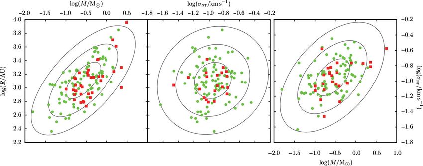
The Role of Discs in Prestellar Cores 3
2010; Green et al. 2011; Principe et al. 2013) can exhibit Table 1. Arithmetic means, standard
large increases in luminosity which last 102 yr. Statistical deviations, and correlation coefficients
arguments by Scholz, Froebrich, & Wood (2013) suggest that of log(M), log(R), and log(σnt ) for
the downtime between outbursts should be of order 104 yr, cores in Ophiuchus.
similar to the timescale given in Equation (3). Parameter Value
μM [log(M/M )] −0.57
3 PRESTELLAR CORES IN OPHIUCHUS μR [log(R/AU)] 3.11
μσ [log(σnt /km s−1 )] −0.95
nt
σM [log(M/M )] 0.43
3.1. Initial conditions
σR [log(R/AU)] 0.27
Using the observed properties of cores as a basis for nu- σσ [log(σnt /km s−1 )] 0.20
nt
merical simulations presents a difficult inverse problem. The ρM,R 0.61
mass, temperature, projected area, and projected aspect ratio ρM,σ 0.49
nt
of a core can be reasonably inferred from bolometric mea- ρR,σ 0.11
nt
surements of the dust in prestellar cores. In addition, the
line-of-sight velocity dispersion within the core can be in-
ferred from the width of molecular lines. However, the initial
boundary conditions of a core simulation must represent the 3.1.2. Shape
full spatial and velocity structure of the system. This occupies
Molecular cloud cores often have elongated, irregular shapes.
six dimensions, whereas observational data can only provide
We include this in the simulations by assuming that each
information on three (i.e. two spatial and one velocity).
intrinsic core shape can be drawn from a family of triaxial
Rather than trying to emulate a specific core—which is
ellipsoids. Each ellipsoid had axes:
arguably an impossibility—we can relatively easily define a
distribution of cores which have the same, or at least very sim- A = 1,
ilar, statistical properties to those in a given region. We based
the synthetic core initial conditions on Ophiuchus. This is a B = exp(τ Gb ), (7)
well-studied region, for which many of the aforementioned C = exp(τ Gc ),
core properties have been measured.
where Gb and Gc are random numbers drawn from a Gaussian
distribution with zero mean and unit standard deviation. The
3.1.1. Mass, size, and velocity dispersion
scale-parameter τ ≈ 0.6 is a fit to the distribution of projected
Only some of the measured core masses in Ophiuchus have aspect ratios in Ophiuchus (Lomax, Whitworth, & Cartwright
both an associated size and velocity dispersion. In order to 2013). The axes are normalised to a given R, giving the
make the most of the data, we define the following lognormal dimensions of the core,
probability distribution of x ≡ (log(M), log(R), log(σnt )):
R
Acore = ,
1 1 T −1 (BC)1/3
P(x) = exp − (x − μ) (x − μ) , (4)
(2π )3/2 || 2 Bcore = BAcore , (8)
where Ccore = CAcore .
⎛ ⎞
μM 3.1.3. Density profile
μ ≡ ⎝ μR ⎠ , (5) Density profiles of cores are often well fitted by those of crit-
μσ
nt ical Bonnor–Ebert spheres (e.g. Bonnor 1956; Alves, Lada,
& Lada 2001; Harvey et al. 2001; Lada et al. 2008). We use
and
such a profile for the ellipsoidal cores. Here, ρ = ρC e−ψ (ξ ) ,
⎛ ⎞ where ρC is the central density, ψ is the Isothermal Function,
σM2 ρM,R σM σR ρM,σ σM σσ
⎜ nt nt ⎟ ξ is the dimensionless radius, ξB = 6.451 is the boundary of
≡ ⎝ ρM,R σM σR σR2 ρR,σ σR σσ
nt ⎠ .
ρM,σ σM σσ ρR,σ σR σσ
nt2
σσ
the sphere. The density at any given point (x, y, z), where
nt nt nt nt nt (0, 0, 0) is the centre of the core, is given by
(6)
The coefficients of μ and are calculated from the observed 1/2
x2 y2 z2
Ophiuchus data (Motte et al. 1998; André et al. 2007) and are ξ = ξFWHM + + , (9)
A2core B2core 2
Ccore
given in Table 1. From P(x), we are able to draw any number
of masses, sizes, and velocity dispersions, all of which were
statistically similar to those in Ophiuchus. The distribution Mcore ξB e−ψ (ξ )
ρ(ξ ) = , ξ < ξB , (10)
of P(x) is shown in Figure 1. 4π Acore BcoreCcore ψ (ξB )
PASA, 33, e004 (2016)
doi:10.1017/pasa.2015.55
Downloaded from https://www.cambridge.org/core. IP address: 46.4.80.155, on 29 Oct 2021 at 12:54:25, subject to the Cambridge Core terms of use, available at https://www.cambridge.org/core/terms.
https://doi.org/10.1017/pasa.2015.554 Lomax et al.
Figure 1. The multivariate lognormal distribution, P(x) where x = (log(M), log(R), log(σnt )). The figure shows the projections through log(σnt ),
through log(M), and through log(R). The concentric ellipses show the 1σ , 2σ, and 3σ regions of the distribution. The green circles are randomly drawn
points from P(x). The red squares are the observational data from Motte et al. (1998) and André et al. (2007). See Lomax et al. (2014) for the original
version of this figure.
where ψ is the first derivative of ψ and ξFWHM = 2.424 is the from accretion (ERF); and finally with continuous feedback
full width at half maximum of the column density through a from accretion (CRF). With CRF, the protostellar luminosity
critical Bonnor–Ebert sphere. was calculated using Equation (2), with Ṁ set to Ṁsink .
3.1.4. Velocity field 3.2.1. Stellar masses
Each core is given a turbulent velocity field with power spec- We find two very noticeable trends when progressing along
trum P ∝ k−4 in three dimensions. We include bulk rota- the series NRF→ERF→CRF. First, the median number
tion and radial excursion by modifying the amplitudes a and stars formed per core decreases: Ns/c nrf = 6.0+4.0 , N erf =
−2.0 s/c
phases ϕ of the k = 1 modes: +3.5 +0.0
⎡ ⎤ ⎡ ⎤
3.5−2.5 , N crf = 1.0−0.0 . Second, the median protostellar
s/c
a(1, 0, 0) rx ωz −ωy mass (see Figure 2) shifts upwards: log10 Mnrf = −1.1+0.4
⎣ a(0, 1, 0) ⎦ = ⎣ −ωz ry −0.6 ,
ωx ⎦ , (11) erf +0.2 crf +0.2 1
log10 M = −0.8−0.4 , log10 M = −0.5−0.2 .
a(0, 0, 1) ωy −ωx rz
These trends occur because disc fragmentation is strongly
⎡ ⎤ ⎡ ⎤ affected by protostellar feedback. In the case with NRF, discs
ϕ(1, 0, 0) π /2 π /2 π /2 are relatively cold and easily fragment. Recall from Equation
⎣ ϕ(0, 1, 0) ⎦ = ⎣ π /2 π /2 π /2 ⎦ . (12) (1) that fragmentation can occur if the disc has a sufficiently
ϕ(0, 0, 1) π /2 π /2 π /2
large column density or the sound speed is sufficiently low.
The amplitude components rx , ry , rz , ωx , ωy , and ωz are drawn With ERF, fragmentation is occasionally interrupted by the
independently from a Gaussian distribution with zero mean episodic outbursts. With CRF, the discs are constantly heated,
and unit variance. The r terms define the amount of excursion and fragmentation becomes difficult. As a consequence, the
along a given axis. The ω terms define the amount rotation central protostar or binary usually accretes the entire mass of
about a given axis. The fields are generated on a 1283 grid and its disc. Protostars with NRF, and to a slightly lesser extent
interpolated onto the SPH particles. The velocity dispersion ERF, are often attended by multiple low-mass companions
of the particles is normalised to a given value of σnt . which partially starve the primary protostar of the remaining
gas. Of the three sets of simulations, those with ERF best
reproduce the Chabrier (2005) IMF.
3.2. Results
In star-forming regions, the observed ratio of stars to brown
One hundred synthetic cores have been evolved for 2 × dwarfs is
105 yr. This is roughly an order of magnitude greater than the N(0.08 M < M ≤ 1.0 M )
average core free-fall time and of the same order as the esti- A= = 4.3 ± 1.6, (13)
N(0.03 M < M ≤ 0.08 M )
mated core–core collisional timescale (André et al. 2007). Of
the one hundred cores, sixty are prestellar. Each simulation
has been performed three times: once with no radiative feed-
back from accretion (NRF); again with episodic feedback 1 The uncertainties give the interquartile range of the distribution.
PASA, 33, e004 (2016)
doi:10.1017/pasa.2015.55
Downloaded from https://www.cambridge.org/core. IP address: 46.4.80.155, on 29 Oct 2021 at 12:54:25, subject to the Cambridge Core terms of use, available at https://www.cambridge.org/core/terms.
https://doi.org/10.1017/pasa.2015.55The Role of Discs in Prestellar Cores 5
Figure 2. The black histograms show stellar mass functions for (a) NRF,
(b) ERF, and (c) CRF. The blue-dotted straight lines, and the red-dashed log- Figure 3. Multiplicity frequency (a), pairing factor (b), and mean system
normal curve, show, respectively, the Chabrier (2005) and Kroupa (2001) fits order (c) for systems with very low mass, M-dwarf and solar-type primaries.
to the observed IMF. The vertical-dashed line shows the hydrogen burning The red boxes give the values for the NRF simulations, blue for the ERF,
limit at M = 0.08 M . See Lomax et al. (2015b) for the original version of and green for the CRF. The black points give the values observed in field
this figure. main-sequence stars. In all cases, the width of a box shows the extent of the
mass bin, and the height shows the uncertainty.
(See Andersen et al. 2008). This figure is best reproduced
with ERF: Aerf = 3.9 ± 0.6.2 Simulations with NRF and fraction of systems which is multiple
CRF yield Anrf = 2.2 ± 0.3 and Acrf = 17 ± 8. While B + T + Q...
mf = , (14)
the figure for NRF is not completely incompatible with ob- S + B + T + Q...
servations, the value with CRF is far too high. This is because
where S is the number of single systems, B is the number of
brown dwarfs are unable to form via disc fragmentation (e.g.
binaries, T is the number of triples, etc. The pairing factor is
Stamatellos, Hubber, & Whitworth 2007a; Stamatellos &
the average number of orbits per system
Whitworth 2009).
B + 2T + 3Q . . .
pf = . (15)
3.2.2. Stellar multiplicities S + B + T + Q...
The core simulations also produce a wide variety of multiple These two quantities are particularly useful in conjunction,
systems. These are either simple binary systems or high order as their ratio gives the average number of objects per multiple
(N ≥ 3) hierarchical multiples. A high-order system can be system
thought of as a binary where one or both components is pf
another binary system. Multiple systems of protostars are Osys = 1 + . (16)
mf
extracted from the end state simulations if they have been
By definition, Osys ≥ 2.
tidally stable for at least one orbital period.
Figure 3 shows mf, pf, and Osys for systems with very
There are many ways to statistically describe the multi-
low mass or brown dwarf primaries, M-dwarf primaries,
plicity of a population of stellar systems. Here, following
and solar-type primaries3 . For comparison, we have also
Reipurth & Zinnecker (1993), we use the multiplicity fre-
quency and the pairing factor. The multiplicity frequency is 3 Here,we define very low mass stars and brown dwarfs as stars with
0.06 M ≤ M < 0.1 M , M-dwarfs as stars with 0.1 M ≤ M < 0.5 M
2 Here, the uncertainty is calculated from the Poison counting error. and solar types as stars with 0.7 M ≤ M < 1.3 M .
PASA, 33, e004 (2016)
doi:10.1017/pasa.2015.55
Downloaded from https://www.cambridge.org/core. IP address: 46.4.80.155, on 29 Oct 2021 at 12:54:25, subject to the Cambridge Core terms of use, available at https://www.cambridge.org/core/terms.
https://doi.org/10.1017/pasa.2015.556 Lomax et al.
Figure 4. A sequence of column density maps of a core during disc fragmentation. The initial core has M = 1.3 M , R = 3000 AU, σnt = 0.3 km s−1
and is evolved with ERF. The colour-bar gives shows the column density in units of g cm−2 . The black dots show the positions of sink particles, i.e.
protostars. Figure 4(a) shows gravitational instabilities developing in a circumbinary disc. Figure 4(b) shows seven protostars in an unstable configuration.
In Figure 4(c), the protostars are configured in a quadruple system (right) and a binary (left); a single protostar is being ejected (centre). Figure 4(d) shows
a stable sextuple system which lasts until the end of the simulation. (a) t = 2.2 × 10⁴ yr (b) t = 2.7 × 10⁴ yr (c) t = 3.2 × 10⁴ yr (d) t = 3.7 × 10⁴ yr
included the same figure for stars in the field (See Duchêne with NRF and ERF. However, with CRF, the multiplicity
& Kraus 2013, and references therein). Observations of pre- frequency is too low for solar-type primaries.
main-sequence stars in Ophiuchus and Taurus suggest that Very high order systems, e.g. sextuples, are also form in
multiplicity is high when stars are young (e.g. Leinert, Zin- these simulations. Figure 4 shows a sextuple system formed
necker, Weitzel, Christou, Ridgway, Jameson, Haas 1993; from a solar mass core with ERF. Initially the core frag-
Ratzka, Köhler, & Leinert 2005; Kraus et al. 2011). As stars ments into two objects, which form a binary system with
age, particularly if they are in a clustered environment, dy- a circumbinary disc. This disc fragments into a further five
namical interactions erode these systems and the multiplicity objects. It finally settles into a sextuple system (a binary
frequency drops to that observed in the field (e.g. Kroupa system orbiting a quadruple) with separations ranging from
1995; Parker et al. 2009; Parker & Goodwin 2011, 2012). ∼ 600 AU for the outer orbit to ∼ 0.1 AU for the innermost
The multiplicity of protostars (i.e. the objects formed in these orbits. Sextuple systems similar to this are found in star-
simulations) should therefore be higher than the multiplicity forming regions (Kraus et al. 2011) and the field Eggleton &
of field stars. This requirement is met for the simulations Tokovinin (2008); Tokovinin (2008).
PASA, 33, e004 (2016)
doi:10.1017/pasa.2015.55
Downloaded from https://www.cambridge.org/core. IP address: 46.4.80.155, on 29 Oct 2021 at 12:54:25, subject to the Cambridge Core terms of use, available at https://www.cambridge.org/core/terms.
https://doi.org/10.1017/pasa.2015.55The Role of Discs in Prestellar Cores 7
All three sets of simulations produce systems with semi- 4.2. Results
major axes ranging between roughly 0.1 AU (the resolution
Figure 5 shows a montage of simulation snapshots where
limit of the simulation) and 1000 AU. This upper limit cor-
the random seed is fixed and δsol is varied from 0 to 1.
responds to that observed in star-forming regions (e.g. King
When the field is purely compressive (δsol = 0), protostars
et al. 2012a, 2012b). Systems with wider orbits ( 103 AU)
form within a network of filaments. Due to the low angular
are probably assembled later through dynamical interactions
momentum of the system, the resultant protostars are only
in clustered environments (e.g. Kouwenhoven et al. 2010).
attended by small discs. In contrast, when the field is purely
solenoidal (δsol = 1), a single protostar forms and is at-
3.3. Summary tended by a coherent disc structure. The disc proceeds to
We find that the mass distribution and multiplicity statistics fragment into multiple objects. A smooth transition between
of young stars can be recovered from simulations if radiative filament fragmentation and disc fragmentation is seen in the
feedback from protostellar accretion is episodic. The periods snapshots with intermediate values of δsol .
of low luminosity provide a window of opportunity, during Figure 6 shows the fraction of protostars formed by fila-
which protostellar discs can fragment. When feedback is ment fragmentation (i.e. in relative isolation) and disc frag-
continuous, the disc is too warm to permit disc fragmentation. mentation (i.e. in discs around more massive protostars) as a
In this instance, the simulations result in (i) a top-heavy IMF, function of δsol . These values are averaged over all random
and (ii) too few stars per core to satisfactorily reproduce seeds. Here, we see that the occurrence of disc fragmentation
observed multiplicity statistics. When there is no radiative increases monotonically with δsol . Filament fragmentation,
feedback, good multiplicity statistics are recovered, but the therefore, decreases monotonically with δsol .
resultant IMF has too many brown dwarfs. On average, the number of protostars spawned per core
ranges from 5.4 ± 7 when δsol = 0 to 8.1 ± 9 when δsol =
1. The median and interquartile range of mass is shown in
4 TURBULENCE: DISCS AND FILAMENTS Figure 7. Here, we see that increasing δsol pushes the me-
To examine how the structure of a core’s velocity field af- dian sink mass down from roughly 0.6 M when δsol = 0 to
fects the star formation process, we take a single core set-up 0.3 M when δsol = 1. We also find that purely compressive
and vary the structure of the velocity field. The core is spheri- fields form very few brown dwarfs. We note that—even for
cal, with M = 3 M , R = 3000 AU, and σnt = 0.44 km s−1 . this limited set of initial conditions—the interquartile range
These dimensions are similar to those of SM1 in Oph-A re- of protostellar masses when δsol 2/3 is very similar to
gion (Motte et al. 1998; André et al. 2007). We alter the that of the Chabrier (2005) IMF.
partition of kinetic energy in solenoidal modes (i.e. shear
and rotation) and compressive modes (i.e. compression and
rarefaction). 4.3. Summary
We show that the collapse and fragmentation of prestellar
4.1. Initial conditions
cores is strongly influenced by the structure of the veloc-
The amplitude of a turbulent mode a(k) can be split into its ity field. Disc formation and fragmentation dominates the
longitudinal (compressive) component al (k) and transverse star formation process when δsol 1/3. At values below
(solenoidal) component at (k) using Helmholtz decomposi- this, stars form mostly through the fragmentation of filamen-
tion: tary structures. The value of δsol also affects distribution
of protostellar masses. The distribution most resembles the
al (k) = k̂(a(k) · k̂),
(17)
observed IMF when δsol 2/3. Reducing δsol reduces
at (k) = a(k) − k̂(a(k) · k̂). the level of disc fragmentation, resulting in smaller number
of objects with greater average mass. In extreme cases (i.e.
When the magnitude and direction of the amplitude is ran- δsol < 1/9), the formation of low-mass stars and brown
dom, there is on average twice as much energy in transverse dwarfs is heavily suppressed. This suggests that disc frag-
modes as there is in solenoidal modes. mentation may be a requirement for forming these objects.
We define the parameter δsol as the average fraction of
solenoidal kinetic energy in a velocity field. We modify the
field to have given δsol by performing the transformation 5 SUMMARY AND CONCLUSIONS
3
a(k) → 3 (1 − δsol ) al (k) + δ a (k). (18) Previous numerical work (e.g. Stamatellos et al. 2007a; Sta-
2 sol t matellos & Whitworth 2009) shows that disc fragmentation
We generate ten initial cores, each with a unique random is important mechanism for reproducing the properties of
velocity seed. For each core, we apply the transformation in low-mass stars. We demonstrate that disc fragmentation also
Equation (18) with values δsol = 0, 19 , 13 , 23 , 1, yielding a plays an important role in the conversion of prestellar cores
total fifty core set-ups. into stars. Importantly, the observed masses and multiplicities
PASA, 33, e004 (2016)
doi:10.1017/pasa.2015.55
Downloaded from https://www.cambridge.org/core. IP address: 46.4.80.155, on 29 Oct 2021 at 12:54:25, subject to the Cambridge Core terms of use, available at https://www.cambridge.org/core/terms.
https://doi.org/10.1017/pasa.2015.558 Lomax et al.
Figure 5. Column density maps of the central 820 AU × 820 AU of the (x, y)-plane, from the simulations with fixed
random seed and different values of δsol , at times t = 1.00, 1.25, 1.50, and 1.75 × 10⁴ yr. The colour scale gives the
logarithmic column density in units of g cm−2 . Sink particles are represented by black dots. See Lomax et al. (2015a)
for the original version of this figure. (a) δsol = 0. (b) δsol = 1/9. (c) δsol = 1/3. (d) δsol = 2/3. (e) δsol = 1.
PASA, 33, e004 (2016)
doi:10.1017/pasa.2015.55
Downloaded from https://www.cambridge.org/core. IP address: 46.4.80.155, on 29 Oct 2021 at 12:54:25, subject to the Cambridge Core terms of use, available at https://www.cambridge.org/core/terms.
https://doi.org/10.1017/pasa.2015.55The Role of Discs in Prestellar Cores 9
tion relative to the observed IMF. Furthermore, filament
fragmentation struggles to produce brown dwarfs and
very low mass stars.
ACKNOWLEDGEMENTS
OL and APW gratefully acknowledge the support of a consoli-
dated grant (ST/K00926/1) from the UK STFC. This work was
performed using the computational facilities of the Advanced Re-
/ / / search Computing @ Cardiff (ARCCA) Division, Cardiff Univer-
sity. All false-colour images have been rendered with splash (Price
Figure 6. The fraction of stars formed by filament fragmentation (red 2007).
crosses) and disc fragmentation (green boxes) for different values of δsol ,
averaged over all random seeds. The error bars show the Poison count-
ing uncertainties. See Lomax et al. (2015a) for the original version of this REFERENCES
figure.
Alves, J. F., Lada, C. J., & Lada, E. A. 2001, Nature, 409, 159
Alves, J., Lombardi, M., & Lada, C. J. 2007, A&A, 462, L17
Andersen, M., Meyer, M. R., Greissl, J., & Aversa, A. 2008, ApJ,
683, L183
André, P., Belloche, A., Motte, F., & Peretto, N. 2007, A&A, 472,
519
Andre, P., Ward-Thompson, D., & Barsony, M. 1993, ApJ, 406, 122
Andre, P., Ward-Thompson, D., & Barsony, M. 2000, Protostars
and Planets IV (Tucson: Univ. Arizona Press), 59
Bate, M. R. 1998, ApJ, 508, L95
Bate, M. R. 2000, MNRAS, 314, 33
/ / /
Bonnor, W. B. 1956, MNRAS, 116, 351
Chabrier, G. 2003, ApJ, 586, L133
Figure 7. The black points show the median stellar mass, and the ver- Chabrier, G. 2005, in Astrophysics and Space Science Library, Vol.
tical black bars show interquartile range of mass, for different values of 327, The Initial Mass Function 50 Years Later, eds. E. Cor-
δsol , averaged over all random seeds. The solid and dashed horizon- belli, F. Palla, H. Zinnecker (Dordrecht: Springrer), p. 41
tal red lines show the median and interquartile range for the Chabrier (arXiv:astro-ph/0409465)
(2005) IMF. See Lomax et al. (2015a) for the original version of this Delgado-Donate, E. J., Clarke, C. J., & Bate, M. R. 2004a, MN-
figure. RAS, 347, 759
Delgado-Donate, E. J., Clarke, C. J., Bate, M. R., & Hodgkin, S. T.
2004b, MNRAS, 351, 617
of stars can be recovered from simulations if the following Duchêne, G., & Kraus, A. 2013, ARA&A, 51, 269
criteria are satisfied: Eggleton, P. P., & Tokovinin, A. A. 2008, MNRAS, 389, 869
Enoch, M. L., Evans, II, N. J., Sargent, A. I., Glenn, J., Rosolowsky,
• Radiative feedback from accretion onto protostars is E., & Myers, P. 2008, ApJ, 684, 1240
Enoch, M. L., et al. 2006, ApJ, 638, 293
episodic. Simulations with episodic radiative feedback
Forgan, D., & Rice, K. 2013, MNRAS, 430, 2082
produce both an IMF and multiplicity statistics in good
Gammie, C. F. 2001, ApJ, 553, 174
agreement with those observed. Simulations with con- Goodwin, S. P., & Whitworth, A. P. 2004, A&A, 413, 929
tinuous radiative feedback fail to produce both the ob- Goodwin, S. P., Whitworth, A. P., & Ward-Thompson, D. 2004,
served number of brown dwarfs and the multiplicity A&A, 423, 169
statistics associated with young objects. Furthermore, Goodwin, S. P., Whitworth, A. P., & Ward-Thompson, D. 2006,
continuous radiative feedback produces protostellar lu- A&A, 452, 487
minosities greater than those observed in young stars. Green, J. D., et al. 2011, ApJ, 731, L25
Simulations with no radiative feedback can produce Greene, T. P., Aspin, C., & Reipurth, B. 2008, ApJ, 135,
good multiplicity statistics and a reasonable—albeit 1421
bottom-heavy—IMF, but are unrealistic. Harvey, D. W. A., Wilner, D. J., Lada, C. J., Myers, P. C., Alves,
J. F., & Chen, H. 2001, ApJ, 563, 903
• A significant proportion of the core’s internal kinetic en-
Hennebelle, P., & Chabrier, G. 2008, ApJ, 684, 395
ergy is in solenoidal turbulent modes. Cores with more
Hennebelle, P., & Chabrier, G. 2009, ApJ, 702, 1428
than a third of their kinetic energy in solenoidal modes Herbig, G. H. 1977, ApJ, 217, 693
are able to easily produce stars via disc fragmentation. Holman, K., Walch, S. K., Goodwin, S. P., & Whitworth, A. P. 2013,
Decreasing this fraction results in more stars forming MNRAS, 432, 3534
in fragmenting filaments. These objects tend to be of Horton, A. J., Bate, M. R., & Bonnell, I. A. 2001, MNRAS, 321,
greater mass, resulting in a top-heavy mass distribu- 585
PASA, 33, e004 (2016)
doi:10.1017/pasa.2015.55
Downloaded from https://www.cambridge.org/core. IP address: 46.4.80.155, on 29 Oct 2021 at 12:54:25, subject to the Cambridge Core terms of use, available at https://www.cambridge.org/core/terms.
https://doi.org/10.1017/pasa.2015.5510 Lomax et al.
Hubber, D. A., Batty, C. P., McLeod, A., & Whitworth, A. P. 2011, Palla, F., & Stahler, S. W. 1993, ApJ, 418, 414
A&A, 529, A27 Parker, R. J., & Goodwin, S. P. 2011, MNRAS, 411, 891
Hubber, D. A., Walch, S., & Whitworth, A. P. 2013, MNRAS, 430, Parker, R. J., & Goodwin, S. P. 2012, MNRAS, 424, 272
3261 Parker, R. J., Goodwin, S. P., Kroupa, P., & Kouwenhoven, M. B. N.
Janson, M., et al. 2012, ApJ, 754, 44 2009, MNRAS, 397, 1577
Johnstone, D., & Bally, J. 2006, ApJ, 653, 383 Pattle, K., et al. 2015, MNRAS, 450, 1094
Johnstone, D., Fich, M., Mitchell, G. F., & Moriarty-Schieven, G. Peneva, S. P., Semkov, E. H., Munari, U., & Birkle, K. 2010, A&A,
2001, ApJ, 559, 307 515, A24
Johnstone, D., Wilson, C. D., Moriarty-Schieven, G., Joncas, G., Price, D. J. 2007, PASA, 24, 159
Smith, G., Gregersen, E., & Fich, M. 2000, ApJ, 545, 327 Principe, D. A., Kastner, J. H., Grosso, N., Hamaguchi, K.,
Kenyon, S. J., & Hartmann, L. 1995, ApJ, 101, 117 Richmond, M., Teets, W. K., & Weintraub, D. A. 2013, preprint
Kenyon, S. J., Hartmann, L. W., Strom, K. M., & Strom, S. E. 1990, (arXiv:1311.5232)
AJ, 99, 869 Raghavan, D., et al. 2010, ApJ, 190, 1
King, R. R., Goodwin, S. P., Parker, R. J., & Patience, J. 2012b, Rathborne, J. M., Lada, C. J., Muench, A. A., Alves, J. F.,
MNRAS, 427, 2636 Kainulainen, J., & Lombardi, M. 2009, ApJ, 699, 742
King, R. R., Parker, R. J., Patience, J., & Goodwin, S. P. 2012a, Ratzka, T., Köhler, R., & Leinert, C. 2005, A&A, 437, 611
MNRAS, 421, 2025 Reipurth, B., & Zinnecker, H. 1993, A&A, 278, 81
Könyves, V., et al. 2010, A&A, 518, L106 Scholz, A., Froebrich, D., & Wood, K. 2013, MNRAS, 430, 2910
Kouwenhoven, M. B. N., Goodwin, S. P., Parker, R. J., Davies, Simpson, R. J., Nutter, D., & Ward-Thompson, D. 2008, MNRAS,
M. B., Malmberg, D., & Kroupa, P. 2010, MNRAS, 404, 1835 391, 205
Kraus, A. L., Ireland, M. J., Martinache, F., & Hillenbrand, L. A. Stamatellos, D., Hubber, D. A., & Whitworth, A. P. 2007a, MN-
2011, ApJ, 731, 8 RAS, 382, L30
Kroupa, P. 1995, MNRAS, 277, 1491 Stamatellos, D., & Whitworth, A. P. 2009, MNRAS, 392, 413
Kroupa, P. 2001, MNRAS, 322, 231 Stamatellos, D., Whitworth, A. P., Bisbas, T., & Goodwin, S. 2007b,
Lada, C. J., Muench, A. A., Rathborne, J., Alves, J. F., & Lombardi, A&A, 475, 37
M. 2008, ApJ, 672, 410 Stamatellos, D., Whitworth, A. P., & Hubber, D. A. 2011, ApJ, 730,
Leinert, C., Zinnecker, H., Weitzel, N., Christou, J., Ridgway, S. T., 32
Jameson, R., Haas, M., & Lenzen, R. 1993, A&A, 278, 129 Stamatellos, D., Whitworth, A. P., & Hubber, D. A. 2012, MNRAS,
Lodato, G., & Rice, W. K. M. 2005, MNRAS, 358, 1489 427, 1182
Lomax, O., Whitworth, A. P., & Cartwright, A. 2013, MNRAS, Stanke, T., Smith, M. D., Gredel, R., & Khanzadyan, T. 2006, A&A,
436, 2680 447, 609
Lomax, O., Whitworth, A. P., & Hubber, D. A. 2015a, MNRAS, Testi, L., & Sargent, A. I. 1998, ApJ, 508, L91
449, 662 Tokovinin, A. 2008, MNRAS, 389, 925
Lomax, O., Whitworth, A. P., Hubber, D. A., Stamatellos, D., & Toomre, A. 1964, ApJ, 139, 1217
Walch, S. 2014, MNRAS, 439, 3039 Tsukamoto, Y., Takahashi, S. Z., Machida, M. N., & Inutsuka, S.
Lomax, O., Whitworth, A. P., Hubber, D. A., Stamatellos, D., & 2015, MNRAS, 446, 1175
Walch, S. 2015b, MNRAS, 447, 1550 Walch, S., Burkert, A., Whitworth, A., Naab, T., & Gritschneder, M.
Matsumoto, T., & Hanawa, T. 2003, ApJ, 595, 913 2009, MNRAS, 400, 13
Morris, J. P., & Monaghan, J. J. 1997, JCoPh, 136, 41 Walch, S., Naab, T., Whitworth, A., Burkert, A., & Gritschneder,
Motte, F., Andre, P., & Neri, R. 1998, A&A, 336, 150 M. 2010, MNRAS, 402, 2253
Motte, F., André, P., Ward-Thompson, D., & Bontemps, S. 2001, Walch, S., Whitworth, A. P., & Girichidis, P. 2012, MNRAS, 419,
A&A, 372, L41 760
Nutter, D., & Ward-Thompson, D. 2007, MNRAS, 374, 1413 Zhu, Z., Hartmann, L., & Gammie, C. 2009, ApJ, 694, 1045
Offner, S. S. R., Klein, R. I., McKee, C. F., & Krumholz, M. R. Zhu, Z., Hartmann, L., & Gammie, C. 2010a, ApJ, 713, 1143
2009, ApJ, 703, 131 Zhu, Z., Hartmann, L., Gammie, C. F., Book, L. G., Simon, J. B.,
Padoan, P., & Nordlund, Å. 2002, ApJ, 576, 870 & Engelhard, E. 2010b, ApJ, 713, 1134
PASA, 33, e004 (2016)
doi:10.1017/pasa.2015.55
Downloaded from https://www.cambridge.org/core. IP address: 46.4.80.155, on 29 Oct 2021 at 12:54:25, subject to the Cambridge Core terms of use, available at https://www.cambridge.org/core/terms.
https://doi.org/10.1017/pasa.2015.55You can also read