The Strength of Absent Ties: Social Integration via Online Dating
←
→
Page content transcription
If your browser does not render page correctly, please read the page content below
The Strength of Absent Ties:
                                                            Social Integration via Online Dating
arXiv:1709.10478v3 [physics.soc-ph] 14 Sep 2018

                                                                    Philipp Hergovich and Josué Ortega∗†

                                                           First version: September 29, 2017. Revised: September 17, 2018.

                                                                                         Abstract

                                                             We used to marry people to whom we were somehow connected.
                                                         Since we were more connected to people similar to us, we were also
                                                         likely to marry someone from our own race.
                                                             However, online dating has changed this pattern; people who meet
                                                         online tend to be complete strangers. We investigate the effects of
                                                         those previously absent ties on the diversity of modern societies.
                                                             We find that social integration occurs rapidly when a society ben-
                                                         efits from new connections. Our analysis of state-level data on in-
                                                         terracial marriage and broadband adoption (proxy for online dating)
                                                         suggests that this integration process is significant and ongoing.

                                                  KEYWORDS: social integration, interracial marriage, online dating, matching in
                                                  networks, random graphs.

                                                  JEL Codes: J12, D85, C78.
                                                     ∗
                                                      Corresponding author: ortega@zew.de ( ).
                                                     †
                                                      Hergovich: University of Vienna. Ortega: Center for European Economic Research
                                                  (ZEW). We are particularly indebted to Dilip Ravindran for his many valuable comments.
                                                  We also acknowledge helpful written feedback from So Yoon Ahn, Andrew Clausen, Melvyn
                                                  Coles, Karol Mazur, David Meyer, Patrick Harless, Misha Lavrov, Franz Ostrizek, Yasin
                                                  Ozcan, Gina Potarca, Reuben Thomas, MSE “quasi” and audiences at the Universities of
                                                  Columbia and Essex, the Paris School of Economics, the Coalition Theory Network Work-
                                                  shop in Glasgow and the NOeg meeting in Vienna. Ortega acknowledges the hospitality of
                                                  Columbia University. Any errors are our own. The corresponding code and data is freely
                                                  available at www.josueortega.com. We have no conflict of interest nor external funding to
                                                  disclose.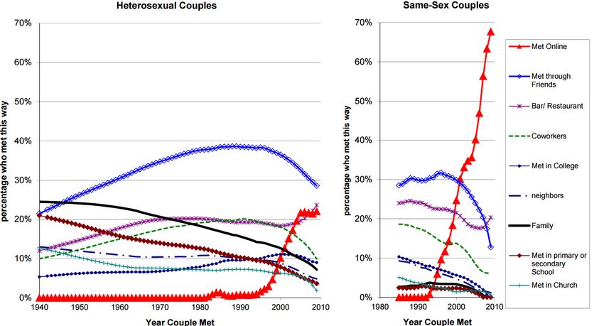
1       Introduction

In the most cited article on social networks,1 Granovetter (1973) argued that
the most important connections we have may not be with our close friends
but our acquaintances: people who are not very close to us, either physically
or emotionally, help us to relate to groups that we otherwise would not be
linked to. For example, it is from acquaintances that we are more likely
to hear about job offers (Rees, 1966; Corcoran, Datcher and Duncan, 1980;
Granovetter, 1995). Those weak ties serve as bridges between our group of
close friends and other clustered groups, hence allowing us to connect to the
global community in a number of ways.2

    Interestingly, the process of how we meet our romantic partners in at
least the last hundred years closely resembles this phenomenon. We would
probably not marry our best friends, but we are likely to end up marrying a
friend of a friend or someone we coincided with in the past. Rosenfeld and
Thomas (2012) show how Americans met their partners in recent decades,
listed by importance: through mutual friends, in bars, at work, in educa-
tional institutions, at church, through their families, or because they became
neighbors. This is nothing but the weak ties phenomenon in action.34

    But in the last two decades, the way we meet our romantic partners
has changed dramatically. Rosenfeld and Thomas argue that “the Internet
increasingly allows Americans to meet and form relationships with perfect
strangers, that is, people with whom they had no previous social tie”. To this
end, they document that in the last decade online dating5 has become the
second most popular way to meet a spouse for Americans (see Figure 1).
    1
      “What are the most-cited publications in the social sciences according to Google?”,
LSE Blog, 12/05/2016.
    2
      Although most people find a job via weak ties, it is also the case that weak ties are
more numerous. However, the individual value from an additional strong tie is larger than
the one from an additional weak tie (Kramarz and Skans, 2014; Gee, Jones and Burke,
2017).
    3
      Backstrom and Kleinberg (2014) reinforce the previous point: given the social network
of a Facebook user who is in a romantic relationship, the node which has the highest
chances of being his romantic partner is, perhaps surprisingly, not the one who has most
friends in common with him.
    4
      Similarly, most couples in Germany met through friends (32%), at the workplace or
school (21%), and bars and other leisure venues (20%) (Potarca, 2017).
    5
      We use the term online dating to refer to any romantic relationship that starts online,
including but not limited to dating apps. We use this terminology throughout the text.

                                             2
Figure 1: How we met our partners in previous decades.
Source: Rosenfeld and Thomas, 2012.
Online dating has changed the way people meet their partners not only
in America but in many places around the world. As an example, Figure
2 shows one of the author’s Facebook friends graph. The yellow triangles
reveal previous relationships that started in offline venues. It can clearly be
seen that those ex-partners had several mutual friends with the author. In
contrast, nodes appearing as red stars represent partners he met through
online dating. These individuals have no contacts in common with him, and
thus it is likely that, if it were not for online dating, they would have never
interacted with him.6
Because a third of modern marriages start online (Cacioppo et al., 2013),
and up to 70% of homosexual relationships, the way we match online with
potential partners shapes the demography of our communities, in particular
its racial diversity. Meeting people outside our social network online can
intuitively increase the number of interracial marriages in our societies, which
is remarkably low. Only 6.3% and 9% of the total number of marriages are
interracial in the US and the UK, respectively.7 The low rates of interracial
6
Although admittedly some of those links may have created after dating, what is clear
is that the author was somewhat connected to these agents beforehand by some mutual
connections, i.e. Granovetter’s weak ties.
7
“Interracial marriage: Who is marrying out”, Pew Research Center, 12/6/2015; and
“What does the 2011 census tell us about inter-ethnic relationships?”, UK Office for
National Statistics, 3/7/2014.
3Figure 2: How one of us met his partners in the last decade.
Triangles are partners met offline, whereas starts are partners met online.
marriage are expected, given that up until 50 years ago these were illegal in
many parts of the US, until the Supreme Court outlawed anti-miscegenation
laws in the famous Loving vs. Virginia case.8
This paper aims at improving our understanding of the impact of online
dating on racial diversity in modern societies. In particular, we intend to find
out how many more interracial marriages, if any, occur after online dating
becomes available in a society. In addition, we are also interested in whether
marriages created online are any different from those that existed before.
Understanding the evolution of interracial marriage is an important prob-
lem, for intermarriage is widely considered a measure of social distance in
our societies (Wong, 2003; Fryer, 2007; Furtado, 2015), just like residential
or school segregation. Moreover, the number of interracial marriages in a
society has important economic implications. It increases the social network
of both spouses who intermarry by connecting them to people of different
race. These valuable connections translate into a higher chance of finding
employment (Furtado and Theodoropoulos, 2010).9 This partially explains
8
Interracial marriage in the US has increased since 1970, but it remains rare (Ar-
row, 1998; Kalmijn, 1998; Fryer, 2007; Furtado, 2015; Chiappori, Oreffice and Quintana-
Domeque, 2016). It occurs far less frequently than interfaith marriages (Qian, 1997).
9
There is a large literature that analyzes the effect of marrying an immigrant. This
literature is relevant because often immigrants are from different races than natives. This
4why the combined income of an White-Asian modern couple is 14.4% higher
than than the combined income of an Asian-Asian couple, and 18.3% higher
than a White-White couple (Wang, 2012). Even when controlling for fac-
tors that may influence the decision to intermarry, Gius (2013) finds that
all interracial couples not involving African Americans have higher combined
incomes than a White-White couple.10
Interracial marriage also affects the offspring of couples who engage in it.
Duncan and Trejo (2011) find that children of an interracial marriage between
a Mexican Latino and an interracial partner enjoy significant human capital
advantages over children born from endogamous Mexican marriages in the
US.11 Those human capital advantages include a 50% reduction in the high
school dropout rate for male children.12
1.1 Overview of Results
This article builds a novel theoretical framework to study matching problems
under network constraints. Our model is different to the previous theoretical
literature on marriage in that we explicitly study the role of social networks
in the decision of whom to marry. Consequently, our model provides new
testable predictions regarding how changes in the structure of agents’ so-
cial networks impact the number of interracial marriages and the quality of
marriage itself. In particular, our model combines non-transferable utility
matching à la Gale and Shapley (1962) with random graphs, first studied by
Gilbert (1959) and Erdős and Rényi (1959), which we use to represent social
networks.13
literature has consistently found that an immigrant who married a native often has a higher
probability of finding employment (Meng and Gregory, 2005; Furtado and Theodoropoulos,
2010; Goel and Lang, 2009). Marrying a native increases the probability of employment,
but not the perceived salary (Kantarevic, 2004).
10
In some cases, intermarriage may even be correlated with poor economic outcomes.
Examining the population in Hawaii, Fu (2007) finds that White people are 65% more
likely to live in poverty if they marry outside their own race.
11
Although Hispanic is not a race, Hispanics do not associate with “standard” races.
In the 2010 US census, over 19 million Latinos identified themselves as being of “some
other race”. See “For many Latinos, racial identity is more culture than color”, New York
Times, 13/1/2012.
12
Pearce-Morris and King (2012) examines the behavioral well-being of children in inter
and intraracial households. They find no significant differences between the two groups.
13
Most of the literature studying marriage with matching models uses transferable util-
ity, following the seminal work of Becker (1973, 1981). A review of that literature appears
5We consider a society composed of agents who belong to different races.
All agents want to marry the potential partner who is closest to them in
terms of personality traits, but they can only marry people who they know,
i.e. to whom they are connected. As in real life, agents are highly connected
with agents of their own race, but only poorly so with people from other
races.14 Again inspired by empirical evidence (Hitsch, Hortasu and Ariely,
2010; Banerjee et al., 2013), we assume that the marriages that occur in our
society are those predicted by game-theoretic stability, i.e. no two unmar-
ried persons can marry and make one better off without making the other
worse off. In our model, there is a unique stable marriage in each society
(Proposition 1).
After computing the unique stable matching, we introduce online dating
in our societies by creating previously absent ties between races and com-
pute the stable marriage again.15 We compare how many more interracial
marriages are formed in the new expanded society that is more interracially
connected. We also keep an eye on the characteristics of those newly formed
marriages. In particular, we focus on the average distance in personality
traits between partners before and after the introduction of online dating,
which we use as a proxy for the strength of marriages in a society (ideally,
all agents marry someone who has the same personality traits as them).
Perhaps surprisingly, we find that making a society more interracially
connected may decrease the number of interracial marriages. It also may
increase the average distance between spouses, and even lead to less married
people in the society (Proposition 2). However, this only occurs in rare cases.
Our main result affirms that the expected number of interracial marriages
in Browning, Chiappori and Weiss (2014). Although our model departs substantially from
this literature, we point out similarities with particular papers in Section 2.
14
The average American public school student has less than one school friend of another
race (Fryer, 2007). Among White Americans, 91% of people comprising their social net-
works are also White, while for Black and Latino Americans the percentages are 83% and
64%, respectively (Cox, Navarro-Rivera and Jones, 2016). Patacchini and Zenou (2016)
document that 84% of the friends of white American students are also white. For high
school students, less than 10% of interracial friendships exist (Shrum, Cheek and Hunter,
1988). Furthermore, only 8% of Americans have anyone of another race with whom they
discuss important matters (Marsden, 1987).
15
We obtain the same qualitative results if we increase both interracial and intraracial
connections, because the marginal value of interracial connections is much larger; see
Appendix B. On a related note, although some dating websites allow the users to sort
partners’ suggestions based on ethnicity, many of them suggest partners randomly. For
our main result, we only need that online daters meet at one partner outside their social
circle. Rosenfeld and Thomas (2012) suggest that this is indeed the case.
6in a society increases rapidly after new connections between races are added
(Result 1). In particular, if we allow marriage between agents who have a
friend in common, complete social integration occurs when the probability
of being directly connected to another race is n1 , where n is the number of
persons in each race. This result provides us with our first and main testable
hypothesis: social integration occurs rapidly after the emergence of online
dating, even if the number of partners that individuals meet from newly
formed ties is small. The increase in the number of interracial marriages in
our model does not require changes in agents’ preferences.
Furthermore, the average distance between married couples becomes smaller,
leading to better marriages in which agents obtain more desirable partners
on average (Result 2). This second result provides another testable hypoth-
esis: marriages created in a society with online dating last longer and report
higher levels of satisfaction than those created offline. We find this hypoth-
esis interesting, as it has been widely suggested that online dating creates
relationships of a lower quality.16 Finally, the added connections in general
increase the number of married couples whenever communities are not fully
connected or are unbalanced in their gender ratio (Result 3). This result pro-
vides a third and final testable hypothesis: the emergence of online dating
leads to more marriages.
We contrast the testable hypotheses generated by the model with US
data. With regards to the first and main hypothesis, we find that the num-
ber of interracial marriages substantially increases after the popularization
of online dating. This increase in interracial marriage cannot be explained
by changes in the demographic composition of the US only, because Black
Americans are the racial group whose rate of interracial marriage has in-
creased the most, going from 5% in 1980 to 18% in 2015 (Livingston and
Brown, 2017). However, the fraction of the US population that is Black has
remained relatively constant during the last 50 years at around 12% of the
population (Pew Reseach Center, 2015).
To properly identify the impact of online dating on the generation of new
interracial marriages, we exploit sharp temporal and geographic variation
in the pattern of broadband adoption, which we use as a proxy for the in-
troduction of online dating. This strategy is sensible given that broadband
adoption has limited correlation to other factors impacting interracial mar-
riages and eliminates the possibility of reverse causation. Using this data
16
“Tinder is tearing society apart”, New York Post, 16/08/2015; and “Online dating is
eroding humanity”, The Guardian, 25/07/11.
7from 2000 to 2016, we conclude that one additional line of broadband inter-
net 3 years ago (marriages take time) affects the probability of being in an
interracial marriage by 0.07%. We obtain this effect by estimating a linear
probability model that includes a rich set of individual- and state-level con-
trols, including the racial diversity of each state and many others. Therefore,
we conclude that there is evidence suggesting that online dating is causing
more interracial marriages, and that this change is ongoing.
Moreover, shortly after we first made available our paper online on Septem-
ber of 2017, Thomas (2018) used recently collected data on how couples meet
to successfully demonstrate that couples that met online are more likely to
be interracial, even when controlling for the diversity of their corresponding
locations. Thomas estimates that American couples who met online since
1996 are 6% to 7% more likely to be interracial than those who met offline.
His findings further establish that online dating has indeed had a positive
impact on the number of interracial marriages, as predicted by our model.
With respect to the quality of marriages created online, both Cacioppo
et al. (2013) and Rosenfeld (2017) find that relationships created online last
at least as long as those created offline, defying the popular belief that mar-
riages that start online are of lower quality than those that start elsewhere,
and are in line with our second prediction (in fact, Cacioppo et al., 2013
finds that marriages that start online last longer and report a higher marital
satisfaction).17
Finally, with respect to our third hypothesis that asserts that online dat-
ing should increase the number of married couples, Bellou (2015) finds causal
evidence that online dating has increased the rate at which both White and
Black young adults marry in the US. The data she analyzes shows that online
dating has contributed to higher marriage rates by up to 33% compared to
the counterfactual without internet dating. Therefore, our third prediction
is consistent with Bellou’s findings.
17
Because online dating is a recent phenomenon, it is unclear whether these effects will
persist in the long run. However, the fact that independent studies find similar effects
suggests that these findings are robust. Rosenfeld (2017) also finds that couples who meet
online marry faster than those created offline.
81.2 Structure of the Article
We present our model in Section 2. Section 3 introduces the welfare indicators
underlying the further analysis. Sections 4 and 5 analyze how these measures
change when societies become more connected using theoretical analysis and
simulations, respectively. Section 6 contrasts our model predictions with
observed demographic trends from the US. Section 7 concludes.
2 Model
2.1 Agents
There are r races or communities, each with n agents (also called nodes).
Each agent i is identified by a pair of coordinates (xi , yi ) ∈ [0, 1]2 , that can be
understood as their personality traits (e.g. education, political views, weight,
height, etcetera).18 Both coordinates are drawn uniformly and independently
for all agents. Each agent is either male or female. Female agents are plotted
as stars and males as dots. Each race has an equal number of males and
females, and is assigned a particular color in our graphical representations.
2.2 Edges
Between any two agents of the same race, there exists a connecting edge
(also called link) with probability p: these edges are represented as solid
lines and occur independently of each other. Agents are connected to others
of different race with probability q: these interracial edges appear as dotted
lines and are also independent. The intuition of our model is that two agents
know each other if they are connected by an edge.19 We assume that p > q.
We present an illustrative example in Figure 3.
18
For a real-life representation using a 2-dimensional plane see
www.politicalcompass.org. A similar interpretation appears in Chiappori, Oref-
fice and Quintana-Domeque (2012) and in Chiappori, McCann and Pass (2016). We use
two personality traits because it allows us to use an illustrative and pedagogic graphical
representation. All the results are robust to adding more personality traits.
19
This interpretation is common in the study of friendship networks, see de Martı́ and
Zenou (2016) and references therein. Our model can be understood as the islands model
in Golub and Jackson (2012), in which agents’ type is both their race and gender.
9Figure 3: Example of a society with n = 4 agents, r = 2 races, p = 1 and
q = 0.2.
Our model is a generalization of the random graph model (Erdős and
Rényi, 1959; Gilbert, 1959; for a textbook reference, see Bollobás, 2001).
Each race is represented by a random graph with n nodes connected among
them with probability p. Nodes are connected across graphs with probability
q. The r random graphs are the within-race set of links for each race. In
expectation, each agent is connected to n(r − 1)q + (n − 1)p persons.
A society S is a realization from a generalized random graph model, de-
fined by a four-tuple (n, r, p, q). A society S has a corresponding graph
S = (M ∪ W ; E), where M and W are the set of men and women, respec-
tively, and E is the set of edges. We use the notation E(i, j) = 1 if there is
an edge between agents i and j, and 0 otherwise. We denote such edge by
either (i, j) or (j, i).
2.3 Agents’ Preferences
All agents are heterosexual and prefer marrying anyone over remaining alone.20
We denote by Pi the set of potential partners for i, i.e. those of different gen-
der. The preferences of agent i are given by a function δi : Pi → R+ that has
20
Both assumptions are innocuous and for exposition only.
10a distance interpretation.21 An agent i prefers agent j ∈ Pi over agent k ∈ Pi
if δi (i, j) ≤ δi (i, k). The intuition is that agents like potential partners that
are close to them in terms of personality traits. The function δi could take
many forms, however we put emphasis on two intuitive ones.
The first one is the Euclidean distance for all agents, so that for any agent
i and every potential partner j 6= i,
q
E
δ (i, j) = (xi − xj )2 + (yi − yj )2 (1)
√
and δ E (i, i) = 2 ∀i ∈ M ∪ W , i.e. the utility of remaining alone equals
the utility derived from marrying the worst possible partner. Euclidean pref-
erences are intuitive and have been widely used in the social sciences (Bogo-
molnaia and Laslier, 2007). The indifference curves associated with Euclidean
preferences can be described by concentric circles around each node.
The second preferences we consider are such that every agent prefers
a partner close to them in personality trait x, but they all agree on the
optimum value in personality trait y. The intuition is that the y-coordinate
indicates an attribute that is usually considered desirable by all partners,
such as wealth. We call these preferences assortative.22 Formally, for any
agent i and every potential partner j ∈ Pi ,
δ A (i, j) = |xi − xj | + (1 − yj ) (2)
and δ E (i, i) = 2 ∀i ∈ M ∪ W . The δ functions we discussed can be
weighted to account for the strong intraracial preferences that are often
observed in reality (Wong, 2003; Fisman et al., 2008; Hitsch, Hortasu and
Ariely, 2010; Rudder, 2014; Potarca and Mills, 2015; McGrath et al., 2016).23
21
The function δ can be generalized to include functions that violate the symmetry
(δ(x, y) 6= δ(y, x)) and identity (δ(x, x) = 0) properties of mathematical distances.
22
If we keep the x-axis fixed, so that agents only care about the y-axis, we get full
assortative mating as a particular case. The preferences for the y attribute are also known
as vertical preferences.
23
It is not clear whether the declared intraracial preferences show an intrinsic intraracial
predilection or capture external biases, which, when removed, leave the partner indifferent
to match across races. Evidence supporting the latter hypothesis includes: Fryer (2007)
documents that White and Black US veterans have had higher rates of intermarriage
after serving with mixed communities. Fisman et al. (2008) finds that people do not find
partners of their own race more attractive. Rudder (2009) shows that online daters have a
roughly equal user compatibility. Lewis (2013) finds that users are more willing to engage
in interracial dating if they previously interacted with a dater from another race.
11Inter or intraracial preferences can be incorporated into the model, as in
equation (3) below
δi0 (i, j) = βij δ(i, j) (3)
where βij = βik if agents j and k have the same race, and βij 6= βik
otherwise. In equation (3), the factor βij captures weightings in preferences.
The case βij < 1 implies that agent i relative prefers potential partners of
the same race as agent j, while βij > 1 expresses relative dislike towards
potential partners of the same race as agent j. Although our results are
qualitatively the same when we explicitly incorporate racial preferences using
the functional form in equation (3), we postpone this analysis to Appendix
B.
A society in which all agents have either all Euclidean or all assortative
preferences will be called Euclidean or assortative, respectively. We focus
on these two cases. In both cases agents’ preferences are strict because we
assume personality traits are drawn from a continuous distribution.
2.4 Marriages
Agents can only marry potential partners who they know, i.e. if there exists
a path of length at most k between them in the society graph.24 We consider
two types of marriages:
1. Direct marriages: k = 1. Agents can only marry if they know each
other.
2. Long marriages: k = 2. Agents can only marry if they know each other
or if they have a mutual friend in common.
To formalize the previous marriage notion, let ρk (i, j) = 1 if there is a
path of at most length k between i and j, with the convention ρ1 (i, i) = 1.
A marriage µ : M ∪ W → M ∪ W of length k is a function that satisfies
∀m ∈ M µ(m) ∈ W ∪ {m} (4)
∀w ∈ W µ(w) ∈ M ∪ {w} (5)
∀i ∈ M ∪ W µ(µ(i)) = i (6)
∀i ∈ M ∪ W µ(i) = j only if ρk (i, j) = 1 (7)
24
A path from node i to t is a set of edges (ij), (jk), . . . , (st). The length of the path is
the number of such pairs.
12We use the convention that agents that remain unmarried are matched to
themselves. Because realized romantic pairings are close to those predicted
by stability (Hitsch, Hortasu and Ariely, 2010; Banerjee et al., 2013), we
assume that marriages that occur in each society are stable.25 A marriage
µ is k-stable if there is no man-woman pair (m, w) who are not married to
each other such that
ρk (m, w) = 1 (8)
δ(m, w) < δ(m, µ(m)) (9)
δ(w, m) < δ(w, µ(w)) (10)
Such a pair is called a blocking pair. Condition (8) is the only non-
standard one in the matching literature, and ensures that a pair of agents
cannot block a direct marriage if they are not connected by a path of length
at most k in the corresponding graph. Given our assumptions regarding
agents’ preferences,
Proposition 1. For any positive integer k, every Euclidean or assortative
society has a unique k-stable marriage.
Proof. For the Euclidean society, a simple algorithm computes the unique k-
stable marriage. Let every person point to their preferred partner to whom
they are connected to by a path of length at most k. In case two people point
to each other, marry them and remove them from the graph. Let everybody
point to their new preferred partner to which they are connected to among
those still left. Again, marry those that choose each other, and repeat the
procedure until no mutual pointing occurs. The procedure ends after at
most rn2
iterations. This algorithm is similar to the one proposed by Holroyd
et al. (2009) for 1-stable matchings in the mathematics literature26 and to
David Gale’s top trading cycles algorithm (in which agents’ endowments
are themselves), used in one-sided matching with endowments (Shapley and
Scarf, 1974) .
For the assortative society, assume by contradiction that there are two
k-stable matchings µ and µ0 such that for two men m1 and m2 , and two
25
We study the stability of the marriages created, following the matching literature, not
of the network per se. Stability of networks was defined by Jackson and Wolinsky (1996)
in the context of network formation. We take the network structure as given.
26
Holroyd et al. (2009) require two additional properties: non-equidistance and no de-
scending chains. The first one is equivalent to strict preferences, the second one is trivially
satisfied. In their algorithm, agents point to the closest agent, independently if they are
connected to them.
13(a) Direct marriage, Euclidean prefer- (b) Long marriage, Euclidean prefer-
ences. ences.
(c) Direct marriage, assortative prefer- (d) Long marriage, assortative prefer-
ences. ences.
Figure 4: Direct and long stable marriages for the Example in Figure 3.
women w1 and w2 , µ(m1 ) = w1 and µ(m2 ) = w2 , but µ0 (m1 ) = w2 and
µ0 (m2 ) = w1 .27 The fact that both marriages are k-stable implies, without
loss of generality, that for i, j ∈ {1, 2} and i 6= j, δ(mi , wi ) − δ(mi , wj ) < 0
and δ(wi , mj ) − δ(wi , mi ) < 0. Adding up those four inequalities, one obtains
0 < 0, a contradiction.
The fact that the stable marriage is unique allows us to unambiguously
compare the characteristics of marriages in two different societies.28 Figure 4
illustrates the direct and long stable marriages for the Euclidean and assor-
tative societies depicted in Figure 3. Marriages are represented as red thick
edges.
27
It could be the case that in the two matchings there are no four people who change
partner, but that the swap involves more agents. The argument readily generalizes.
28
In general, the set of stable marriages is large. Under different restrictions on agents’
preferences we also obtain uniqueness (Eeckhout, 2000; Clark, 2006). None of the restric-
tions mentioned in those papers applies the current setting.
142.5 Online Dating on Networks and Expansions of So-
cieties
We model online dating in a society S by increasing the number of interracial
edges. Given the graph S = (M ∪ W ; E), we create new interracial edges
between every pair that is disconnected with a probability .29,30 S denotes
a society that results after online dating has occurred in society S. S has
exactly the same nodes as S, and all its edges, but potentially more. We say
that the society S is an expansion of the society S. Equivalently, we model
online dating by increasing q. Online dating generates a society drawn from
a generalized random graph model with a higher q, i.e. with parameters
(n, r, p, q + ).
3 Welfare Indicators
We want to understand how the welfare of a society changes after online
dating becomes available, i.e. after a society becomes more interracially
connected. We consider three welfare indicators:
1. Diversity, i.e. how many marriages are interracial. We normalize this
indicator so that 0 indicates a society with no interracial marriages, and 1
equals the diversity of a colorblind society in which p = q, where an expected
fraction r−1
r
of the marriages are interracial. Formally, let R be a function
that maps each agent to their race and M ∗ be the set of married men. Then
|{m ∈ M ∗ : R(m) 6= R(µ(m))}| r
dv(S) = ∗
· (11)
|M | r−1
√
2. Strength, defined as 2 minus the average Euclidean distance between
each married couple. This number is normalized to be between 0 and 1. If
29
Online dating is likely to also increase the number of edges inside each race, but since
we assume that p > q, these new edges play almost no role. We perform robustness checks
in Appendix B, increasing both p and q but keeping its ratio fixed.
30
We could assume that particular persons are more likely than others to use online
dating, e.g. younger people. However, the percentage of people who use online dating has
increased for people of all ages. See: “5 facts about online dating”, Pew Research Center,
29/2/2016. To obtain our main result, we only need a small increase in the probability of
interconnection for each agent.
15every agent gets her perfect match, strength is 1, but if every agent marries
the worst possible partner, strength equals 0. We believe strength is a good
measure of the quality of marriage not only because it measures how much
agents like their spouses, but also because a marriage with a small distance
between spouses is less susceptible to break up when random agents appear.
Formally
√ P
δ E (m,µ(m))
2 − m∈M ∗|M ∗ |
st(S) = √ (12)
2
3. Size, i.e. the ratio of the society that is married. Formally,
|M ∗ |
sz(S) = (13)
n
4 Edge Monotonicity of Welfare Indicators
Given a society S, the first question we ask is whether the welfare indicators
of a society always increase when its number of interracial edges grow, i.e.
when online dating becomes available. We refer to this property as edge
monotonicity.31
Definition 1. A welfare measure w is edge monotonic if, for any society S,
and any of its extensions S , we have
w(S ) ≥ w(S) (14)
That a welfare measure is edge monotonic implies that a society unam-
biguously becomes better off after becoming more interracially connected.
Unfortunately,
Proposition 2. Diversity, strength, and size are all not edge monotonic.
Proof. We show that diversity, strength and size are not edge monotonic
by providing counterexamples. To show that size is not edge monotonic,
31
Properties that are edge monotonic have been thoroughly studied in the graph theory
literature (Erdős, Suen and Winkler, 1995). Edge monotonicity is different from node
monotonicity, in which one node, with all its corresponding edges, is added to the matching
problem. It is well-known that when a new man joins a stable matching problem, every
woman weakly improves, while every man becomes weakly worse off (Theorems 2.25 and
2.26 in Roth and Sotomayor, 1992).
16consider the society in Figure 3 and its direct stable matching in Figure
4a. Remove all interracial edges: it is immediate that in the unique stable
matching there are now four couples, one more than when interracial edges
are present.
For the case of strength, consider a simple society in which all nodes
share the same y-coordinate, as the one depicted in Figure 5. There are
two intraracial marriages and the average Euclidean distance is 0.35. When
we add the interracial edge between the two central nodes, the closest nodes
marry and the two far away nodes marry too. The average Euclidean distance
in the expanded society increases to 0.45, hence reducing its strength.
Figure 5: Strength is not edge monotonic.
The average Euclidean distance between spouses increases after creating the interracial
edge between the nodes in the center.
To show that diversity is not edge monotonic, consider Figure 6. There
are two men and two women of each of two races a and b. Each gender is
represented with the superscript + or − .
Stability requires that µ(b− + + −
1 ) = a1 and µ(b2 ) = a2 , and everyone else is
−
unmarried. However, when we add the interracial edge (a+ 1 b2 ), the married
couples become µ(b− + + − + −
1 ) = b1 , µ(a2 ) = a1 , and µ(a1 ) = b2 . In this extended
society, there is just one interracial marriage, out of a total of three, when
before we had two out of two. Therefore diversity reduces after adding the
−
edge (a+1 b2 ).
The failure of edge monotonicity by our three welfare indicators makes
evident that, to evaluate welfare changes in societies, we need to understand
how welfare varies in an average society after introducing new interracial
edges. We develop this comparison in the next Section.
A further comment on edge monotonicity. The fact that the size of a
society is not edge monotonic implies that adding interracial edges may not
lead to a Pareto improvement for the society. Some agents can become worse
17(a) dv(S) = 2 (b) dv(S ) = 2/3
Figure 6: Diversity is not edge monotonic.
−
The diversity of this society reduces after creating the interracial edge (a+
1 , b2 ). The top
graph represents the original society. The bottom left graph show the marriages in the
original society, whereas the bottom right graph shows the marriages in the expanded
society.
off after the society becomes more connected. Nevertheless, the fraction of
agents that becomes worse off after adding an extra edge is never more than
one-half of the society, and although it does not vanish as the societies grow
large, the welfare losses measured in difference in spouse ranking become
asymptotically zero. ? discusses both findings in detail.
5 Expected Welfare Indicators
To understand how the welfare indicators behave on average, we need to
form expectations of these welfare measures. We are able to evaluate this
expression analytically for diversity, and rely on simulation results for the
18others.
5.1 Diversity
The expected diversity of a society with direct marriages is given by
q (r−1)n
2 r
E[dv(Sdirect )] = · (15)
p n2 + q (r−1)n
2
r−1
where q(r − 1)n/2 is the expected number of potential partners of a dif-
ferent race to which an agents is directly connected, and pn/2 is the corre-
sponding expected number of potential partners of the same race. The term
r
r−1
is just the normalization we impose to ensure that diversity equals one
when p = q. Equation (15) is a concave function of q, because
∂ 2 E[dv(Sdirect )] −pr(r − 1)
2
=Plugging the values computed in equations (18) and (19) into (17), we can
plot that function and observe that it grows very fast: after q becomes pos-
itive, the diversity of a society quickly becomes approximately one. To un-
derstand the rapid increase in diversity, let us fix p = 1 and let q = 1/n.
Then
P (B) = 1 − (1 − q)2n−1 (1 − q 2 )(r−2)n (20)
= 1 − (1 − q)rn−1 (1 + q)(r−2)n (21)
1 1
= 1 − (1 − )rn−1 (1 + )(r−2)n (22)
n n
= 1 − e−2 ≈ 0.86 (23)
n→∞
Substituting the value of P (B) into (17), we obtain that E[dv(Slong )] ≈
.86r
.86r+.14
which is very close to 1 even when r is small (E[dv(Slong )] ≈ .92
,
already for r = 2), showing that the diversity of a society becomes 1 for very
small values of q, in particular q = 1/n. The intuition behind full diversity
for the case of long marriages is that, once an agent obtains just one edge to
any other race, he gains n2 potential partners. Just one edge to a person of
different race gives access to that person’s complete race.
Although we fixed p = 1 to simplify the expressions of expected diversity,
the rapid increase in diversity does not depend on each race having a complete
graph. We also obtain a quick increase in diversity for many other values of p,
as we discuss in Appendix B. When same-race agents are less interconnected
among themselves, agents gain fewer connections once an interracial edge is
created, but those fewer connections are relatively more valuable, because
the agent had less potential partners available to him before.32
To further visualize the rapid increase in diversity we use simulations.
We generate several random societies and observe how their average diversity
change when they become more connected. We create ten thousand random
societies, and increase the expected number of interracial edges by increasing
32
This finding should not be confused with (and it is not implied by) two well-known
properties of random graphs. The first one establishes that a giant connected component
emerges in a random graph when p = 1/n, whereas the graph becomes connected when
p = log(n)/n; for a review of these properties see Albert and Barabási (2002). The second
result is that the property that a random graph has diameter 2 (maximal path length
between nodes) has a sharp threshold at p = (2 ln n/n)1/2 (Blum, Hopcroft and Kannan,
2017). Result 1 is also similar to, but not implied by, the small world property of simple
random graphs (Watts and Strogatz, 1998), where an average small path length occurs in
a regular graph after rewiring a few initial edges.
20the parameter q. In the simulations presented in the main text we fix n = 50
and p = 1.33
As predicted by our theoretical analysis, a small increase in the probabil-
ity of interracial connections achieves perfect social integration in the case
of long marriages.34,35 For the cases with direct marriages, the increase in
diversity is slower but still fast: an increase of q from 0 to 0.1 increases diver-
sity to 0.19 for r = 2, and from 0 to 0.37 with r = 5.36 Figure 7 summarizes
our main result, namely:
Result 1. Diversity is fully achieved with long marriages, even if the increase
in interracial connections is arbitrarily small.
With direct marriages, diversity is achieved partially, yet an increase in
q around q = 0 yields an increase of a larger size in diversity.
We have showed that with either direct (k = 1) or long (k = 2) marriages
diversity increases after the emergence of online dating, although at very
different rates. An obvious question is whether online dating actually helps
to create long marriages. We study the case of long marriages not because
we expect that if a man meets a woman online, then that man will be able
to date that woman’s friends. Rather, we study it because it shows that
when people meet their potential spouses via friends of friends (k > 2), a
few existing connections can quickly make a difference: recall that meeting
through friends of friends is the most common way to meet a spouse both
in the US and Germany (around one out of every three marriages start this
way in both countries (Rosenfeld and Thomas, 2012; Potarca, 2017)).37
Our analysis shows that immediate social integration occurs for all values
of k ≥ 2. The mechanism we consider for those larger values of k is that, once
33
We restrict to n = 50 and ten thousand replications because of computational limi-
tations. The results for other values of p are similar and we describe them in Appendix
B.
34
Perfect social integration (diversity equals one) occurs around q = 1/n, as we have
discussed. The emergence of perfect integration is not a phase transition but rather a
crossover phenomenon, i.e. diversity smoothly increases instead of discontinuously jumping
at a specific point: see Figure B1 in Appendix B.
35
This result is particularly robust as it does not depend on our assumption that the
marriages created are stable. Stability is not innocuous in our model, as we could consider
other matching schemes that in fact are edge-monotonic.
36
Empirical evidence strongly suggests that q is very close to zero in real life. See
footnote 13.
37
Ortega (2018b) finds the minimal number of interracial edges needed to guarantee that
any two agents can marry for all values of k.
21Figure 7: Average diversity of an Euclidean society for different values of q.
The yellow and orange curves are indistinguishable in this plot because they are identical.
Exact values and standard errors (which are in the order of 1.0e-04) are provided in
Appendix A, as well as the corresponding graph for an assortative society, which is almost
identical.
an interracial couple is created, it serves as a bridge between two different
races. For example, if woman a marries man b of a different race, in the
future it allows agent a0 , an acquaintance of woman a, to meet agent b0 , an
acquaintance of man b, allowing a0 and b0 to marry. In summary, we expect
that some marriages created by online dating will be between people who
meet directly online, but some will be created as a consequence of those
initial first marriages, and thus the increase in the diversity of societies will
be somewhere in between the direct and the long marriage case.
Result 1 implies that a few interracial links can lead to a significant
increase in the racial integration of our societies, and leads to optimistic
views on the role that dating platforms can play in modern civilizations.
Our result is in sharp contrast to the one of Schelling (1969, 1971) in its
seminal models of residential segregation, in which a society always becomes
completely segregated. We pose this finding as the first testable hypothesis
of our model.
Hypothesis 1. The number of interracial marriages increases after the pop-
ularization of online dating.
225.2 Strength & Size
A second observation, less pronounced than the increase in diversity, is that
strength is increasing in q. We obtain this result by using simulations only,
given that it seems impossible to obtain an analytical expression for the
expected strength of a society.38 Figure 8 presents the average strength of
the marriages obtained in ten thousand simulations with n = 50 and p = 1.
Figure 8: Average strength of an Euclidean society for different values of q.
Exact values and standard errors (which are in the order of 1.0e-04) provided in Appendix
A, as well as the corresponding graph for an assortative society, which is very similar.
The intuition behind this observation is that agents have more partner
choices in a more connected society. Although this does not mean that every
agent will marry a more desired partner, it does mean that the average agent
will be paired with a better match. It is clear that, for all combinations
of parameters (see Appendix B for further robustness checks), there is a
consistent trend downwards in the average distance of partners after adding
new interracial edges, and thus a consistent increase in the strength of the
societies. We present this observation as our second result.
38
Solving the expected average distance in a toy society with just one race, containing
only one man and one woman, requires a long and complicated computation “Distance
between two random points in a square”, Mind your Decisions, 3/6/2016.
23Result 2. Strength increases after the number of interracial edges increases.
The increase is faster with long marriages and with higher values of r.
Assuming that marriages between spouses who are further apart in terms
of personality traits have a higher chance of divorcing because they are more
susceptible to break up when new nodes are added to the society graph, we
can reformulate the previous result as our second hypothesis.
Hypothesis 2. Marriages created in societies with online dating have a lower
divorce rate.
Finally, with regards to size, we find that the number of married people
also increases when q increases. This observation, however, depends on p <
1.39 This increase is due to the fact that some agents do not know any
available potential spouse who prefers them over other agents. Figure 9
presents the evolution of the average size of a society with p = 1/n.
The increase in the number of married people becomes even larger (and
does not require p < 1) whenever i) some races have more men than women,
and vice versa,40 ii) agents become more picky and are only willing to marry
an agent if he or she is sufficiently close to them in terms of personality traits,
or iii) some agents are not searching for a relationship. All these scenarios
yield the following result.
Result 3. Size increases after the number of interracial edges increases if
either p < 1, societies are unbalanced in their gender ratio, or some agents
are deemed undesirable. The increase is faster with long marriages and with
higher values of r.
The previous result provides us with a third and final testable hypothesis,
namely:
Hypothesis 3. The number of married couples increases after the popular-
ization of online dating.
39
Using Hall’s marriage theorem, Erdős and Rényi (1964) find that in a simple random
graph (r = 1) the critical threshold for the existence of a perfect matching is p = log n/n,
i.e. a marriage with size 1. Even when p = q, this critical threshold is only a lower bound
for a society to have size 1. This is because there is no guarantee that the stable matching
will in fact be a perfect one.
40
See Ahn (2018) for empirical evidence on how gender imbalance affects cross-border
marriage.
24Figure 9: Average size of an Euclidean society for values of q up to p = 1/n.
Exact values and standard errors (which are in the order of 1.0e-04) provided in Appendix
A, as well as the corresponding graph for an assortative society, which is very similar.
6 Hypotheses and Data
6.1 Hypothesis 1: More Interracial Marriages
What does the data reveal? Is our model consistent with observed demo-
graphic trends? We start with a preliminary observation before describing
our empirical work in the next subsection. Figure 10 presents the evolu-
tion of interracial marriages among newlyweds in the US from 1967 to 2015,
based on the 2008-2015 American Community Survey and the 1980, 1990
and 2000 decennial censuses (IPUMS). In this Figure, interracial marriages
include those between White, Black, Hispanic, Asian, American Indian or
multiracial persons.41
We observe that the number of interracial marriages has consistently in-
creased in the last 50 years. However, it is intriguing that a few years after
the introduction of the first dating websites in 1995, like Match.com, the
41
We are grateful to Gretchen Livingston from the Pew Research Center for providing
us with the data. Data prior to 1980 are estimates. The methodology on how the data
was collected is described in Livingston and Brown (2017).
25Figure 10: Percentage of interracial marriages among newlyweds in the US.
Source: Pew Research Center analysis of 2008-2015 American Community Survey and
the 1980, 1990 and 2000 decennial censuses (IPUMS). The red, green, and purple lines
represent the creation of Match.com, OKCupid, and Tinder. The creation of Match.com
roughly coincides with the popularization of broadband in the US and the 1996 Telecom-
munications Act. The blue line represents a linear prediction for 1996 – 2015 using the
data from 1967 to 1995.
percentage of new marriages created by interracial couples increased. The
increase becomes steeper around 2006, a couple of years after online dating
became more popular: it is around this time when well-known platforms such
as OKCupid emerged. During the 2000s, the percentage of new marriages
that are interracial rose from 10.68% to 15.54%, a huge increase of nearly 5
percentage points, or 50%. After the 2009 increase, the proportion of new
interracial marriage jumps again in 2014 to 17.24%, remaining above 17% in
2015 too. Again, it is interesting that this increase occurs shortly after the
creation of Tinder, considered the most popular online dating app.42
The increase in the share of new marriages that are interracial could be
caused by the fact that the US population is in fact more interracial now
42
Tinder, created in 2012, has approximately 50 million users and produces more than
12 million matches per day. See “Tinder, the fast-growing dating app, taps an age-old
truth”, New York Times, 29/10/2014. The company claims that 36% of Facebook users
have had an account on their platform.
26than 20 years ago. However, the change in the population composition of
the US cannot explain the huge increase in intermarriage that we observe, as
we discuss in detail in Appendix C. A simple way to observe this is to look
at the growth of interracial marriages for Black Americans. Black Americans
are the racial group whose rate of interracial marriage has increased the
most, going from 5% in 1980 to 18% in 2015. However, the fraction of
the US population that is Black has remained constant at around 12% of
the population during the last 40 years. Random marriage accounting for
population change would then predict that the rate of interracial marriages
would remain roughly constant, although in reality it has more than tripled
in the last 35 years.
The correlation between the increase in the number of interracial mar-
riages and the emergence of online dating is suggestive, but the rise of inter-
racial marriage may be due to many other factors, or a combination of those.
To precisely pin down the effect of online dating in this increase, we proceed
as follows.
6.2 Empirical Test of Hypothesis 1
We use the following strategy in order to rigorously test our prediction that
online dating increases the number of interracial marriages. Our empirical
setup exploits state variations in the development of broadband internet from
2000 to 2016, which we use as a proxy for online dating. There is little concern
for reverse causality, which would imply that broadband developed faster in
states where there was a higher number of interracial couples. Our dependent
variable is a dummy showing whether a person’s marriage is interracial. We
use a variety of personal and state-level covariates in order to identify the
relationship between online dating and interracial marriages as precisely as
possible. Figure 11 displays a preview of the relationship between broadband
development and interracial marriage by state.
We use three main data sources for our analysis. All data concerning in-
dividuals is downloaded from IPUMS, and we restrict our analysis to married
individuals only. Although the data is only on the individual level, it is possi-
ble to construct marriage relationships, by employing a matching procedure
described at IPUMS website. As additional control variables, we employ ed-
ucation, age, and total income,43 as these are likely to affect the marriage
43
One might worry about endogeneity coming from income, as the marriage decision
27Figure 11: Change in % of marriages that are interracial in US, by state.
Source: FCC statistical reports on broadband development, US Census population
estimates, and the American Community Survey (IPUMS) from 2000 to 2016.
decision.
We construct the broadband data using information from reports by the
Federal Communications Commission (FCC), which is the regulatory author-
ity in the United States responsible for communication technology. Following
Bellou (2015),44 we use the number of residential high-speed internet lines
per 100 people as our explanatory variable. Data is available for the years
2000 to 2016. However, we have to discard Hawaii from our analysis, as
observations are missing up to 2005.
We download additional state controls from the Current Population Sur-
vey. Following Bellou’s work, we include variables like the ratio of the male
divided by female population within a state, age bins and the ratio of non-
white people in a state. This last explanatory variable is especially important
in our context of interracial marriages.
might affect earnings. Excluding income as explanatory variable leaves the coefficients
virtually unchanged. As additional robustness check, we estimate a similar model at state
level in Appendix D.
44
She uses a similar specification to examine the role of internet diffusion in the creation
of new marriages. Our dataset is described in detail in Appendix D.
28We estimate the following reduced form equation by a linear probability
model:
Interist = α + β Broadbandst + γ1 Xist + γ2 Zst + F Es + F Et + ist (24)
where Interist is one if a person is in an interracial marriage and 0 other-
wise. The indices relate to person i, living in state s at time t. We are mostly
interested in the coefficient β, as it captures the propensity of online dating.
The values in X are covariates relating directly to the person, while Z rep-
resents time varying state variables. We additionally include state- and year
fixed effects, and cluster the standard errors ist at the state-year level. Our
rich battery of control variables enables us to clearly identify the relationship
between interracial marriages and broadband internet, which can be seen as
an instrument for online dating. As marriages take a while to form, we in-
clude the broadband variable with a 3 year lag based on empirical evidence
(Rosenfeld, 2017).45
The first column in Table 1 states that one additional line of broadband
internet 3 years ago affects the probability of being in an interracial marriage
by 0.07%. The coefficient is positive, as predicted by our theoretical model.
In column (2) we include controls at the state level and find that the rela-
tionship between interracial marriages and broadband remains significantly
positive. This continues to be true when including the individual covari-
ates, all of which decrease the probability of a marriage being interracial.
Perhaps surprisingly, education enters negatively. A potential underlying
reason might be that education leads to more segregated friendship circles,
a conjecture worth being explored in subsequent work.
Column (4) is now the specification outlined in (24). Even with all con-
trols, the effect of broadband penetration on interracial marriages is highly
significant and positive. This result suggests a causal relationship in the
sense described by our model. As additional evidence for this claim, we
see that once we replace the lagged broadband with its contemporaneous
counterpart, the coefficient declines in size, which means that the state of
45
In Appendix D we follow a different strategy. We construct shares of interracial
marriages per state and year and estimate this with panel methods. The advantage is
that the dependent variable is continuous rather than dichotomous, however we cannot use
individual controls and introduce standard errors via aggregation. These standard errors
should be negligible given the amount of observations we have available. The state-year
level specification also generates significant coefficients with the expected signs, confirming
our results.
29You can also read