The study of variability in engineering design-An appreciation and a retrospective
←
→
Page content transcription
If your browser does not render page correctly, please read the page content below
Data-Centric Engineering (2021), 2: e3
        doi:10.1017/dce.2021.3

        PERSPECTIVE

        The study of variability in engineering design—An
        appreciation and a retrospective
        Timothy Peter Davis*
        Department of Statistics, University of Warwick, Coventry, United Kingdom
        *Corresponding author. E-mail: tim@timdavis.co.uk
        Received: 24 March 2021; Revised: 29 March 2021; Accepted: 06 April 2021
        Keywords: Robustness; parameter design; transmitted variation; statistical engineering

        Abstract
        We explore the concept of parameter design applied to the production of glass beads in the manufacture of metal-
        encapsulated transistors. The main motivation is to complete the analysis hinted at in the original publication by Jim
        Morrison in 1957, which was an early example of discussing the idea of transmitted variation in engineering design,
        and an influential paper in the development of analytic parameter design as a data-centric engineering activity.
        Parameter design is a secondary design activity focused on selecting the nominals of the design variables to achieve
        the required target performance and to simultaneously reduce the variance around the target. Although the 1957 paper
        is not recent, its approach to engineering design is modern.

           Impact Statement
           This paper draws attention to a 1957 publication by Jim Morrison and illustrates the concept of parameter design
           (a secondary design activity between concept design and tolerance design). The 1957 paper was the first in the
           English language to discuss parameter design and is an early example of data-centric engineering. This paper
           illustrates that the obvious or intuitive solutions to design optimization can be wrong, even in the simplest of
           cases as illustrated here, motivating the need for careful data-centered analysis, when solving engineering
           problems.

        1. Introduction
        The concept of engineering design robustness has been well established since the work of Japanese
        engineer Genichi Taguchi became known in the western economies in the 1980s, for example, Taguchi
        and Wu (1985) and subsequently Taguchi (1986).
           Design robustness is formulating a design with a functional response that is as immune as possible to
        so-called noise factors.1

           1
             Noise factors are sources of variation (either environmental variables or manufacturing variation in design variables) that affect
        the response. Noise factors are variables that the design engineer cannot control or chooses not to control. Robustness is the task of

        © The Author(s), 2021. Published by Cambridge University Press. This is an Open Access article, distributed under the terms of the Creative Commons
        Attribution-NonCommercial-ShareAlike licence (http://creativecommons.org/licenses/by-nc-sa/4.0/), which permits non-commercial re-use,
        distribution, and reproduction in any medium, provided the same Creative Commons licence is included and the original work is properly cited.
        The written permission of Cambridge University Press must be obtained for commercial re-use.

Downloaded from https://www.cambridge.org/core. 10 Sep 2021 at 04:34:30, subject to the Cambridge Core terms of use.
e3-2         Timothy Peter Davis

           The challenge of design robustness has been around for a long time and was uppermost in the minds of
        18th century engineers, for example, John Harrison in his design of a clock that could keep time despite
        humidity, and the rolling motion of a ship, to solve the longitude problem, and Josiah Wedgewood in
        making good quality China pieces, despite variability of temperature inside his kilns, although the word
        robustness was not common parlance at that time.
           Many decades prior to the awareness of Taguchi’s work a seminal paper was published by Jim
        Morrison2 who addressed a particular type of robustness problem, that of transmitted variation (Morrison,
        1957). At the time Morrison was working as a glass engineer for the British Thomson–Houston company
        in Rugby UK. This early paper addressed a key problem of robustness associated with the manufacture of
        encapsulated transistors.

        2. The Glass Beads Problem
        This problem arose in the early days of semiconductors, whereby development work was proceeding on a
        new range of metal-encapsulated transistors. The envelope comprised a metal disk to which the
        germanium or silicon wafer would be attached and a flanged metal “top hat” which would be welded
        to the disk to complete the enclosure. The electrical connections to the transistor consisted of two fine
        wires which were sealed into flanged holes on the disk by fusing glass beads to form a hermetic seal. (see
        Figure 1). This problem provided the motivation for the 1957 paper.
            Although this case study is not recent, it is modern. Its main teaching point as we will see, is that the
        “obvious” (to the uninitiated) solution to this simple problem is wrong, which motivates application of
        Morrison’s method to more complicated problems, whereby the solution will not in any sense be obvious.
            It is worth noting that the small glass beads are not just parts but are part of something (a bigger
        system—e.g., the complete circuit hardware). Often the performance of an entire system relies heavily on
        the performance of the smallest parts, for example, in the case of the 1986 Challenger disaster—see
        Feynman (1986).
            After the 1957 paper surfaced (due in large part to the work of George Box and his colleagues at the
        Center for Quality and Productivity Improvement at the University of Wisconsin3), Morrison pub-
        lished a coda to the 1957 paper (Morrison, 1998), where he introduced the term variance synthesis and
        described his general approach as statistical engineering.4 To quote directly from the 1998 paper “the
        concept of transmitted error was implicit in the 1957 article, yet it remained neglected and undeve-
        loped until the early 1980s when Taguchi and Wu (1985) introduced off-line quality control and Box
        and Fung (1986) showed that in suitable circumstances, the error transmission formula provided a
        better approach…(than those proposed by Taguchi and Wu)” Additionally, the 1998 paper gave more
        detail on how the glass beads were made, which we repeat here verbatim to provide context for the
        study.

            “Because of the low volume of this special glass, the glass was melted in a small pot and the longer
            glass tubes from which the beads were cut, were then “drawn” by hand. A skilled glass blower
            would gather a quantity of molten glass on the end of a blow pipe and would “marver” it to a
            cylindrical shape on a flat metal plate after putting a puff of air into the gather to keep it hollow, A
            co-worker would then stick a “punty” on the opposite end of the gather and the two would then walk
            backwards away from each other along a tube-drawing alley.

        achieving a functional response on target with minimal variation around the desired target, despite the presence of these noise
        factors.
           2
             I knew both Genichi Taguchi, and Jim Morrison, and learned much from them both.
           3
             Indeed, it was George Box’s work at the Center for Quality Improvement at the University of Wisconsin in the mid 1980s that
        drew this author’s attention to the 1957 paper. For a collection of much of the Center’s work in this area and at this time see the
        collected works in Box (2000) in particular Part E (Variance reduction and robustness) pages 429–552.
           4
             Morrison introduced the term Statistical Engineering in some of his earlier publications.

Downloaded from https://www.cambridge.org/core. 10 Sep 2021 at 04:34:30, subject to the Cambridge Core terms of use.
Data-Centric Engineering   e3-3

        Figure 1. A diagram of a single bore bead together with a metal-encapsulated transistor. The glass bead
                    (left figure) ends up inside the “top hat” enclosing the transistor (right figure).

            A third colleague armed with a board would fan the glass to cool it until the tubing was thought to be
            the right size.5 The tubing was then cut up into lengths of about 1 m prior to shipping to the
            customer.”

        There were several types of glass beads mentioned in the 1957 paper: A standard wall bead, a thick wall
        bead, and a triple-bore bead, but following Morrison (1957), the focus of our discussion is on the standard-
        wall bead—see Figure 1.
           The volume of a single bore bead is given by the following objective function.6

                                                         π D2  B2 L
                                                     V¼                                                          (1)
                                                               4
        There are three relevant dimensions (the outer diameter ½D, the inner bore ½B, and the length ½L) and
        these are, collectively the design variables. Table 1 shows the measurements of these dimensions taken on
        a sample of 30 beads, carefully measured with a measurement microscope.
            The volumes in Table 1 were estimated from the volume equation (1) and were calibrated by estimating
        the volumes by weighing (ignoring any variation in glass density). The volume estimates derived from the
        glass density, were on average lower than those calculated geometrically, primarily due to the beads not
        being perfectly circular, and some of the beads losing some material by being chipped (a failure mode
        which we ignore in this paper).
            There were two distinct failure modes which hampered high-quality production of the beads. Firstly,
        the glass beads would crack under temperature gradients due to the differences in thermal properties of the
        glass and the metal of the mounting surface that was being sealed. A so-called one-sided failure mode
        (Clausing and Frey, 2005). Secondly, at the preproduction stage, a high failure rate was being experienced
        in the glass/metal sealing process because the volume of the glass in production was too variable. For
        example, (a) if the volume of the glass bead was too great, the fused glass would spread across the disk and
        impede the mounting of the wafer at the next production stage and (b) if the volume was too small, surface
        tension would pull the glass to one side leaving a gap in the seal meaning the seal was not airtight. This is a
        two-sided failure mode illustrated in Figure 2 and is the main focus of this paper.
            Both failure modes are caused by noise factors. In the glass cracking case, the noise factor is an
        environmental variable (temperature), and in the excessive glass volume variability case, the noise factor
        is variation in the design variables which is transmitted to the volume.
            The countermeasure for the glass cracking was to make the glass from a special borosilicate
        composition whose expansion characteristics matched those of the metal it was sealing, so that the seal
        would be stress free (in other words robust to temperature).
            With regard to the variability that is transmitted from an input variable x say, to an output variable y say,
        is given by the expression σ 2y ≈ ∂y
                                          ∂x σ x , where the derivative of the objective function is evaluated at the point
                                               2

           5
             This account explains why variability was a concern in the production of these beads! A YouTube video on making glass
        cylinders can be found at https://www.youtube.com/watch?v=-eFAeHuGaG4.
           6
             Sometimes called a transfer function.

Downloaded from https://www.cambridge.org/core. 10 Sep 2021 at 04:34:30, subject to the Cambridge Core terms of use.
e3-4         Timothy Peter Davis

        Table 1. The mean dimensions and variances of a sample of 30 beads, as reported in Morrison (1957).

        Bead dimension                                               Sample mean x1                                            Sample variance S 2xi

        D                                                              xD ¼ 1:96mm                                              S 2D ¼ 0:00125mm2
        B                                                             xB ¼ 0:625mm                                              S 2B ¼ 0:00254mm2
        L                                                               xL ¼ 1:92mm                                             S 2L ¼ 0:00536mm2
        Bead volume ðV Þ                                               V ¼ 3:72mm3                                               S 2V ¼ 0:0617mm3
        The volumes in Table 1 were estimated from the volume equation (1) and were calibrated by estimating the volumes by weighing (ignoring any
        variation in glass density). The volume estimates derived from the glass density, were on average lower than those calculated geometrically, primarily
        due to the beads not being perfectly circular, and some of the beads losing some material by being chipped (a failure mode which we ignore in this
        paper).

          Figure 2. Figure reproduced with permission from the Chartered Quality Institute. This figure first
        appeared in the January 1998 edition of Quality World, in the article “Looking Back” by Jim Morrison.

        of interest in the x space (usually the nominal or target value, such that when x takes this value, the required
        output value y is achieved. The expression is of course exact if the relationship between y and x is linear,
        and will provide an adequate approximation if y ¼ f ðxÞ is roughly linear in a near-neighborhood of x:7
            When there is more than one design variable, there usually is, say fxi gki¼1. In the glass bead example,
        there are three design variables, fxi g3i¼1 ¼ fD,B, Lg, and so the variance transmission formula is
        (assuming the xi s are independent8)
                                                          X3  ∂y 2
                                                   σ 2y ¼    i¼1 ∂x
                                                                         :σ 2xi ,                                    (2)
                                                                     i

        where the derivatives are calculated at the nominals for the xi s. we take the nominal values as the mean
        values in Table 1. The partial derivatives are easily derived and so equation (2) (with V taking the role of y)
        becomes
                                                2           2          2
                                                ∂V             ∂V           ∂V
                                         σV ¼
                                          2
                                                       σD þ
                                                        2
                                                                     σB þ
                                                                      2
                                                                                  σ 2L ,                           (3)
                                                ∂D             ∂B           ∂L

           7
            Morrison (1957) suggests that equation (2) will be adequate as long as the standard deviation is less than 20% of the mean.
           8
            In the 1957 account, Morrison indicates that there is “a slight degree of correlation” between B an D. Unfortunately, the original
        data are no longer available to check the value of this correlation, but we investigate the consequences of such a correlation, based on
        plausible assumptions, further on in the paper.

Downloaded from https://www.cambridge.org/core. 10 Sep 2021 at 04:34:30, subject to the Cambridge Core terms of use.
Data-Centric Engineering   e3-5

                                                                      2     2
                                                   πDL 2 2    πBL 2 2    π D  B2
                                         σ 2V   ¼       σD þ       σB þ               σ 2L ,                                  (3a)
                                                    2          2             4
        so
                                  σ 2V ¼ ð25:98  0:00125Þ þ ð3:55  0:00254Þ þ ð3:75  0:00536Þ,                             (3b)
        and finally,
                                                σ 2V ¼ 0:0325 þ 0:0090 þ 0:0201 ¼ 0:0617 mm6 :                                (3c)
        Note that each derivative has units mm4 So that these equations are dimensionally consistent.
            Observe that it is the diameter D that accounts for most of the variability transmitted to V, and not L
        even though σ 2L > σ 2D . This is because the gradient in the direction of D (25.98) is much greater than in the
        direction L (3.75). This example shows that even in such a simple case, the “obvious” solution of attacking
        the design variable with the largest variance is wrong. It can only be speculated as to how intuition might
        let us down in more complicated examples.
            Before this analysis was done by Jim Morrison, The British Thomson-Houston Company, Ltd. (which
        was part of GE) was planning to spend a lot of money investing in a new cutting machine to improve the
        accuracy of the cut length (L) of the beads.
            It turned out that the reduction in the variance of the diameter was easier to achieve than reduction in the
        variance of the length because it was observed that D only varied gradually along a cut length of glass
        tubing of ~1 m in length.
            By cutting these longer 1-m lengths into shorter pieces of ~10 cm and producing batches of beads from
        these shorter lengths, the variability of D within a batch of these 10 cm lengths was reduced which in turn
        resulted in a large reduction in the variance of the glass bead volume. This clever control plan based on
        sorting the shorter batches bypassed the need for new cutting equipment to control cut length L, since the
        glass beads were easily batched according to their origin from the shorter pieces.9
            The glass bead example nicely illustrates the importance of analyzing transmitted variation in making
        the right engineering and manufacturing decisions to improve quality and avoid unnecessary cost.
            The analysis of transmitted variation was called tolerance design by Taguchi (1986). Jim Morrison
        came to call this variance synthesis (Morrison, 1998).
            Tolerance design is a tertiary design activity—the primary design activity is establishing the basic
        design concept to deliver the functionality as required by the customer or end-user.
            A secondary design activity is choosing the correct nominals for the design variables, so that the
        objective target is achieved. If the secondary design activity also has the objective of improving design
        robustness (minimizing transmitted variation), then Taguchi called this parameter design.
            In his 1957 paper, Jim Morrison did not pursue a parameter design solution for the glass beads,
        although a careful reading of the paper did show that he had thought about it: “In situations in which bead
        volume is a critical factor, the designer can use this analysis as a guide in determining the most suitable
        proportions of bead for a given application.”
            Bisgaard and Ankemann (2005) claim that this is the first reference to parameter design in the
        literature. So, we look at parameter design in some detail now.

        3. A Parameter Design Study of the Glass Beads
        The parameter design problem for the glass beads can be stated as minimize the transmitted variation
        given by (3) subject to V ¼ 3:72 mm (equation (1)). Here, we use the Solver function in MS Excel® to
        determine the solution.

          9
            It may be tempting to think that these days sorting to achieve high quality is not required. But even in high precision
        manufacturing sorting can be effective, for example, in the fitting of fan blades to modern jet engines.

Downloaded from https://www.cambridge.org/core. 10 Sep 2021 at 04:34:30, subject to the Cambridge Core terms of use.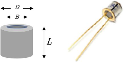
e3-6          Timothy Peter Davis

          Table 2. The initial design specification prior to conducting parameter design, with the resulting
                                                 transmitted variation.

                               Initial design                                                                               Variance transmitted
                               specification
                                                            Variance
                                                        Assumed                                 Assumed                             to
                                                                                                                  σ
        Dimension                    μx i                     σ 2xi                      coefficient of variation μxi       V from equation (3)
                                                                                                                      xi

                                                                               2
        D                         1:69 mm                   0.00125 mm                                0.02092                    0.0325 mm6
        B                        0:625 mm                   0.00254 mm2                               0.00806                    0.0090 mm6
        L                        1:92 mm                    0.00536 mm2                               0.03813                    0.0201 mm6
        Volume (V)               3:72 mm3                                                                                        0.0616 mm6

                                                       Table 3. The parameter design solution.

                                Design specification
                                  after parameter
                                                                                                           Coefficient            Variance
                                                                                                                           σ
        Dimension                  design μxi                         Assumed Variance σ 2xi                  of variation μxi    transmitted to V
                                                                                                                            xi

                                                                                                  2
        D                                2:0 mm                               0.00175 mm                         0.02092           0.0293 mm6
        B                                0:6 mm                               0.00234 mm2                        0.00806           0.0035 mm6
        L                               1:30 mm                               0.00246 mm2                        0.03813           0.0201 mm6
        Volume (V)                      3:72 mm3                                                                                   0.0529 mm6
        Note that the coefficients of variation are as in Table 2 per our assumption, that is, σ xi ∝ μxi .

             We make some realistic assumptions before proceeding; firstly, we assume a constant coefficient of
                      σ
        variation μxi for each of the three design variables fxi g3i¼1 ¼ fD,B, Lg since in engineering and manufactur-
                        xi
        ing applications, it is often true that the variability and the mean are linked. A general link function is
        σ xi ∝ μpxi , where a constant coefficient of variation corresponds to the case p ¼ 1. But other values of p may
        be appropriate (see Box, 1988). We begin by assuming that p ¼ 1. The coefficients of variation can be
        calculated directly from Table 1. Secondly, we add the constraint that the bore dimension B, must be in the
        interval (0.60.65 mm), so that the thin wires can pass through the bead easily. Also, the diameter
        D clearly needs to be greater than the bore, so D >, and it cannot be too large, otherwise the bead will not
        locate into the “top hat,” so we arbitrarily set the constraint D ≤ 2 mm.
             We take as the starting values or initial design specification the measurements given in Morrison
        (1957). These are summarized in Table 2.
             After running the Excel solver with the constraints as specified, the results are as given in Table 3. Note
        the coefficients of variation are the same in each case per our assumption.
             Note that comparing the postparameter design in Table 3 with the initial specification in Table 2, the
        transmitted variation has reduced from 0:0616 to 0:0529 or about 14%. This gain is equivalent to reducing
        the variance of D in the initial specification by about 20%. Note in Table 3 the changes in the nominal
        values for D, B, and L compared to Table 2. Figure 3 illustrates the parameter design solution graphically.
             Note from Figure 3 that the optimal value of the outer diameter D is on the edge of its constraint, so if
        this constraint could be relaxed, for example, by using a larger “top hat,” a better solution (i.e., a further
        reduction in σ 2V ) could be realized.10
             It has long been recognized that the importance of the assumption regarding the relationship between
        μxi and σ xi is crucial in parameter design. For example, if we repeat the previous analysis, but now assume

           10
                The diameter of a glass tube is a function of the speed at which the glass is drawn.

Downloaded from https://www.cambridge.org/core. 10 Sep 2021 at 04:34:30, subject to the Cambridge Core terms of use.
Data-Centric Engineering e3-7
Figure 3. Contours of transmitted variation from bead dimensions D and L to volume V under the
assumption that σ xi ∝ μxi . The red line corresponds to V ¼ 3:72 mm. In this plot, the bore diameter B is set
to its optimal value of 0.6 mm. The open dot is the initial specification (slightly off the red line because
initially B 6¼ 0:6), and the solid dot is the parameter design solution.
Table 4. Parameter design solution assuming that the variances of the bead dimensions are fixed at the
values given in Table 2.
Parameter design
Variance assumed
Variance transmitted
Dimension xi nominal μxi fixed σ 2xi to V
D 1:74 mm 0.00175 mm2 0.0294 mm6
B 0:6 mm 0.00234 mm2 0.0071 mm6
L 1:77 mm 0.00246 mm2 0.0236 mm6
Volume ðV Þ 3:72 mm3 0.0601 mm6
Note from Table 4 that the proposed nominals for D and L are quite different to the previous solution. This sensitivity of the parameter design method
was acknowledged by Morrison (1957) and was discussed more extensively by Box and Fung (1994). The contour plot under the assumption of fixed
variances for D, B, and L is shown in Figure 4.
that the variances for the bead dimensions are fixed at the values in Table 1 (i.e., p ¼ 0), the parameter
design solution is as in Table 4.
Additionally, to the functional relationship between σ xi and μxi , we should also check for the effect of a
lack of independence between the design variables. Morrison (1957) hints that variables B and D were
slightly correlated (larger bores tended to result in larger outer diameters). If we denote the correlation
between B and D by ρDB an additional term must be added to the variance transmission formula, (3),
namely
∂V ∂V π 2 BDL2
2 : σ B σ D ρDB ¼ :σ B σ D ρDB :
∂B ∂D 2
Downloaded from https://www.cambridge.org/core. 10 Sep 2021 at 04:34:30, subject to the Cambridge Core terms of use.e3-8 Timothy Peter Davis
Figure 4. Contours of the transmitted variation now assuming fixed variances for the bead dimensions,
showing the new parameter design solution (solid dot), compared to the previous solution under the
assumption of constant coefficient of variation (the solid square, now with σ 2V ¼ 0:068470). The initial
design specification is shown by the open dot. Note that the contours in Figure 4 are oriented differently
compared to those in Figure 3, illustrating the sensitivity of parameter design to underlying assumptions,
to the extent that optimal value of the outer diameter D is now well within the imposed constraint. Clearly
in this case, and in general, the functional relationship between σ xi and μxi needs to be carefully
established.
Table 5. The consequences of a correlation between design variables (in this case D and B).
p ¼ 0 (i.e., σ xi is fixed) p ¼ 1 (i.e., σ xi ∝ μxi )
σ 2V with fD, B, Lg Contribution σ 2V with fD,B,Lg Contribution
ρBD of ρDB to σ 2V of ρDB to σ 2V
0:0 0.060079 {1.74,0.6,1.77} 0.0 0.052896 {2,0.6,1.3} 0.0
0:1 0.062911 {1.76,0.6,1.73} 0.0018 0.054926 {2,0.6,1.3} 0.0020
0:2 0.065633 {1.78,0.6,1.69} 0.0036 0.056956 {2,0.6,1.3} 0.0041
0:3 0.068259 {1.80,0.6,1.65} 0.0054 0.058986 {2,0.6,1.3} 0.0061
Note that when p ¼ 0, the optimal values for D and L depend on ρDB , due to the orientation of the contours, so this highlights that the independence of the
design variables needs to be considered in parameter design studies in addition to the considerations emphasized in Box and Fung (1994).
Note that with this extra term equation (3) is still dimensionally consistent.
The results in Table 5 illustrate the effects of a weak correlation between B and D (say ρBD ≤ 0:3). Note
that the optimal value for the design variables only change when p ¼ 0, and the transmitted variation to
V increases with ρBD . The orientation of the contours of transmitted variation do not change with ρDB ,
so we do not show them here.
One other approach to deal with correlated variables in a parameter design study is to express
the objective function in dimensionless variables using an application of Buckingham’s “Pi theorem”
Downloaded from https://www.cambridge.org/core. 10 Sep 2021 at 04:34:30, subject to the Cambridge Core terms of use.Data-Centric Engineering e3-9
Figure 5. The parameter design solution with ρDB ¼ 0 and p ¼ 0 for D and B, and p ¼ 1 for L. The optimal
values for fD,B,Lg are f2:0,0:6,1:3g, with σ 2V ¼ 0:044830. As in the previous figures the open dot is the
initial bead specification and the parameter design solution by the solid dot.
(e.g., see Shen et al., 2014). For the objective function (1), if we take as our dimensionless variables,
π 0 ¼ BV3 , π 1 ¼ DB, and π 2 ¼ BL, then π 0 ∝ π 21 1 : π 2 : The dimension of the problem is reduced by one. Note
that the two variables which exhibit a correlation now appear as a ratio. Grove and Davis (1992) show how
dimensionless variables help with parameter design by exploring this idea while analyzing Taguchi’s
celebrated and widely taught Wheatstone Bridge problem (see Box, 2000, Chapter E.3), albeit in that case
to deal with an interaction between design variables rather than a correlation.
Determining a value for p from the summary data for fD,B, Lg regarding the three types of beads
discussed in the 1957 paper is inconclusive, but there is some evidence that for D and B, p ¼ 0, while for L,
p ¼ 1. To conclude the parameter design discussion, we investigate the effect that this hybrid assumption
has on the parameter design solution.
Firstly assuming ρDB ¼ 0 to allow for direct comparison to the solutions illustrated in Figures 3 and 4,
the resulting contour plot is shown in Figure 5. The optimal value for σ 2V is now 0:44830:
Note that in Figure 5, the orientation of the contours is similar to Figure 3 when it was assumed that ¼ 1
∀fD, B,Lg, so it is the variance assumption on L which dictates the re-orientation of the contours observed
in Figure 4.
Exploring this hybrid assumption now for the range of values for ρDB that were considered previously,
we find the results in Table 6. Note that although the optimal values of fD, B,Lg do not alter from the
assumption of p ¼ 1 for each design variable, the optimal value for σ 2V is improved from the previous
results.
In summary, we see that for the glass bead study it is the assumption regarding the link between σ L and
μL that is crucial for this analysis on three counts—the orientation of the contours and the optimal settings
for fD, B,Lg and magnitude of the transmitted variance.
4. In Retrospect
Morrison’s (1957) paper was it seems the first paper to formulate the idea of parameter design although he
did not call it that and he did not explore that idea in his paper. Together with the fact that he published the
Downloaded from https://www.cambridge.org/core. 10 Sep 2021 at 04:34:30, subject to the Cambridge Core terms of use.e3-10 Timothy Peter Davis
Table 6. Parameter design solution under the assumption p ¼ f0, 0, 1g for fD,B, Lg for various values
of ρDB .
Optimal fD, B,Lg Contribution
ρBD for p ¼ f0,0, 1g σ 2V of ρDB to σ 2V
0:0 f2:0,0:6, 1:3g 0.044830 0.0
0:1 f2:0,0:6, 1:3g 0.046615 0.0018
0:2 f2:0,0:6, 1:3g 0.048403 0.0036
0:3 f2:0,0:6, 1:3g 0.050190 0.0054
paper in a journal that engineers do not usually read, may explain why Morrison’s early ideas were not
picked up in the engineering mainstream until the work of Taguchi became better known. Subsequently
George Box and his co-workers at the Center for Quality and productivity improvement at the University
of Wisconsin-Madison regularly referenced the 1957 paper in their many publications.
The method was used in the Ford Motor Company (Parry-Jones, 1999; Davis, 2006) as part of a
coordinated strategy to embed robust design into engineering practice and was taught in company training
programs.
It is hoped that as more data-centric engineering methods (Girolami, 2020) are developed as part of the
statistical engineering framework, Morrison’s work with suitable modern adaptions will find continue to
find its place in current engineering design challenges. Although the glass bead example is simple to
understand, the solution to reducing the transmitted variation is not obvious, which has implications for
applications with many more design variables. Recent developments in applying parameter design for
situations that rely on a computer model (a “digital-twin”) to evaluate design alternatives, because an
explicit objective function is not available due to complexity and high dimension, is given in Shen (2017).
In his 1998 coda to the 1957 paper, Morrison laid out a 11-step process for reducing variability in
engineering design. The final step was (my italics).
“The possibility of experimenting with the nominal values of the design parameters … can be explored
especially if the variances are not constant but alter with changes in the nominal values.”
The analysis of the glass beads problem presented here illustrates step 11 for the glass beads problem
and emphasizes the importance of checking the assumptions regarding the way in which the standard
deviation and mean of the design variables may be linked.
The purpose of this paper is to recognize and honor the importance of Jim Morrison’s paper as a
foundational paper for statistical engineering, and to investigate the parameter design solution to the glass
bead problem that Morrison envisaged but did not actually do. My one regret is that I did not do this
sooner, so that I could have shared this work with him.11
Funding Statement. This work received no specific grant from any funding agency, commercial or not-for-profit sectors.
Competing Interests. The author declares no competing interests exist.
Data Availability Statement. Data availability is not applicable to this article as no new data were created or analyzed in this study.
Author Contributions. T.P.D. is the sole contributor to this work. There are no competing interests to declare and likewise there is
no funding to declare. The data referred to in Table 1 are not available.
Acknowledgments. I would like to thank Dr. Shirley Coleman, of Newcastle University, Jon Bridges of the University of Bradford,
and an anonymous referee for making constructive comments on an earlier draft.
11
Jim Morrison’s obituary can be found in Journal of the Royal Statistical Society Series A, 180(1), 348–350 and online at https://
rss.onlinelibrary.wiley.com/doi/full/10.1111/rssa.12271.
Downloaded from https://www.cambridge.org/core. 10 Sep 2021 at 04:34:30, subject to the Cambridge Core terms of use.Data-Centric Engineering e3-11
References
Bisgaard S and Ankenman A (1995) Analytical parameter design. Quality Engineering 8(1), 75–91.
Box GEP (1988) Signal-to-noise ratios, performance criteria, and transformations. Technometrics 30(1), 1–39.
Box GEP (2000) Tiao GC, Bisgaard S, Hill WJ, Pena D and Stigler SM (eds), Box on Quality and Discovery, with Design, Control,
and Robustness. New York: Wiley.
Box GEP and Fung CA (1986) Studies in Quality Improvement: Minimising Transmitted Variation by Parameter Design,
Technical Report No. 8. Madison, WI: Center for Quality and Productivity Improvement.
Box GEP and Fung CA (1994) Is your robust design procedure robust? Quality Engineering 9(3), 503–514. https://minds.
wisconsin.edu/bitstream/handle/1793/69173/r008.pdf?sequence=1&isAllowed=y, (accessed 28 April 2021).
Clausing D and Frey DD (2005) Improving system reliability by failure-mode avoidance including four concept design strategies.
Systems Engineering 8(3), 245–261.
Davis TP (2006) Science engineering and statistics. Applied Stochastic Models in Business and Industry 22(5–6), 401–430.
Feynman RP (1986) Personal Observations on the Reliability of the Shuttle. Appendix F, Report of the Presidential Commission on
the Space Shuttle Challenger Accident. Washington, DC: Rogers WP (Chair), US Government, Rogers Commission. https://
history.nasa.gov/rogersrep/v2appf.htm, (accessed 28 April 2021).
Girolami M (2020). Introducing Data-Centric Engineering: an open access journal dedicated to the transformation of engineering
design and practice. Data-Centric Engineering Journal 1, e1.
Grove DM and Davis TP (1992) Engineering Quality and Experimental Design. Harlow: Longman.
Morrison SJ (1957) The study of variability in engineering design. Applied Statistics 6(2), 133–138.
Morrison SJ (1998) Variance synthesis revisited. Quality Engineering 11(1), 149–155.
Parry-Jones R (1999) Engineering for Corporate Success in the New Millennium. Westminster, UK: Royal Academy of
Engineering.
Shen W (2017) Robust parameter designs in computer experiments using stochastic approximation. Technometrics 59(4), 471–483.
Shen W, Davis TP, Lin D and Nachtsheim C (2014) Dimensional analysis and its applications in statistics. Journal of Quality
Technology 46(3), 185–198.
Taguchi G (1986) System of Experimental Design. Vols. 1 & 2. New York: Unipub/Kraus International.
Taguchi G and Wu Y-I (1985) Introduction to Off-Line Quality Control. Nagoya, Japan: Central Japan Quality Control
Association.
Cite this article: Davis T. P (2021). The study of variability in engineering design—An appreciation and a retrospective. Data-
Centric Engineering, 2: e3. doi:10.1017/dce.2021.3
Downloaded from https://www.cambridge.org/core. 10 Sep 2021 at 04:34:30, subject to the Cambridge Core terms of use.You can also read