Towards Generalization and Simplicity in Continuous Control
←
→
Page content transcription
If your browser does not render page correctly, please read the page content below
Towards Generalization and Simplicity
                                                               in Continuous Control

                                                  Aravind Rajeswaran∗         Kendall Lowrey∗       Emanuel Todorov        Sham Kakade
                                                                             University of Washington Seattle
arXiv:1703.02660v2 [cs.LG] 20 Mar 2018

                                                        { aravraj, klowrey, todorov, sham } @ cs.washington.edu

                                                                                        Abstract
                                                    This work shows that policies with simple linear and RBF parameterizations can
                                                    be trained to solve a variety of widely studied continuous control tasks, including
                                                    the OpenAI gym benchmarks. The performance of these trained policies are com-
                                                    petitive with state of the art results, obtained with more elaborate parameterizations
                                                    such as fully connected neural networks. Furthermore, the standard training and
                                                    testing scenarios for these tasks are shown to be very limited and prone to over-
                                                    fitting, thus giving rise to only trajectory-centric policies. Training with a diverse
                                                    initial state distribution induces more global policies with better generalization.
                                                    This allows for interactive control scenarios where the system recovers from large
                                                    on-line perturbations; as shown in the supplementary video.

                                         1   Introduction
                                         Deep reinforcement learning (deepRL) has recently achieved impressive results on a number of
                                         hard problems, including sequential decision making in game domains [1, 2]. This success has
                                         motivated efforts to adapt deepRL methods for control of physical systems, and has resulted in rich
                                         motor behaviors [3, 4]. The complexity of systems solvable with deepRL methods is not yet at the
                                         level of what can be achieved with trajectory optimization (planning) in simulation [5, 6, 7], or with
                                         hand-crafted controllers on physical robots (e.g. Boston Dynamics). However, RL approaches are
                                         exciting because they are generic, model-free, and highly automated.
                                         Recent success of RL [2, 8, 9, 10, 11] has been enabled largely due to engineering efforts such
                                         as large scale data collection [1, 2, 11] or careful systems design [8, 9] with well behaved robots.
                                         When advances in a field are largely empirical in nature, it is important to understand the relative
                                         contributions of representations, optimization methods, and task design or modeling: both as a
                                         sanity check and to scale up to harder tasks. Furthermore, in line with Occam’s razor, the simplest
                                         reasonable approaches should be tried and understood first. A thorough understanding of these factors
                                         is unfortunately lacking in the community.
                                         In this backdrop, we ask the pertinent question: "What are the simplest set of ingredients needed
                                         to succeed in some of the popular benchmarks?" To attempt this question, we use the Gym-v1 [12]
                                         continuous control benchmarks, which have accelerated research and enabled objective comparisons.
                                         Since the tasks involve under-actuation, contact dynamics, and are high dimensional (continuous
                                         space), they have been accepted as benchmarks in the deepRL community. Recent works test their
                                         algorithms either exclusively or primarily on these tasks [13, 4, 14], and success on these tasks have
                                         been regarded as demonstrating a “proof of concept”.

                                         Our contributions: Our results and their implications are highlighted below with more elaborate
                                         discussions in Section 5:
                                             ∗
                                                 Equal contributions. Project page: https://sites.google.com/view/simple-pol

                                         31st Conference on Neural Information Processing Systems (NIPS 2017), Long Beach, CA, USA.
1. The success of recent RL efforts to produce rich motor behaviors have largely been attributed
to the use of multi-layer neural network architectures. This work is among the first to carefully
analyze the role of representation, and our results indicate that very simple policies including
linear and RBF parameterizations are able to achieve state of the art results on widely studied tasks.
Furthermore, such policies, particularly the linear ones, can be trained significantly faster (almost
20x) due to orders of magnitude fewer parameters. This indicates that even for tasks with complex
dynamics, there could exist relatively simple policies. This opens the door for studying a wide
range of representations in addition to deep neural networks and understand trade-offs including
computational time, theoretical justification, robustness, sample complexity etc.
2. We study these issues not only with regards to the performance metric at hand but we also take
the further step in examining them in the context of robustness. Our results indicate that, with
conventional training methods, the agent is able to successfully learn a limit cycle for walking,
but cannot recover from any perturbations that are delivered to it. For transferring the success of
RL to robotics, such brittleness is highly undesirable.
3. Finally, we directly attempt to learn more robust policies through using more diverse train-
ing conditions, which favor such policies. This is similar in spirit to the model ensemble
approaches [15, 16] and domain randomization approaches [17, 18], which have successfully
demonstrated improved robustness and simulation to real world transfer. Under these new and
more diverse training scenarios, we again find that there is no compelling evidence to favor the
use of multi-layer architectures, at least for the benchmark tasks. On a side note, we also provide
interactive testing of learned policies, which we believe is both novel and which sheds light on
the robustness of trained policies.
Overall, we note that this work does not attempt to provide a definitive answer in terms of the
ideal architecture choice for control. Rather, the results in this work suggest that the current set of
benchmark tasks are insufficient to provide insights to this question. We further note that as the
research field progresses, it is imperative to revisit these questions to make well calibrated progress.
2 Problem Formulation and Methods
We consider Markov Decision Processes (MDPs) in the average reward setting, which is defined using
the tuple: M = {S, A, R, T , ρ0 }. S ⊆ Rn , A ⊆ Rm , and R : S × A → R are a (continuous) set of
states, set of actions, and reward function respectively, and have the usual meaning. T : S × A → S
is the stochastic transition function and ρ0 is the probability distribution over initial states. We wish
to solve for a stochastic policy of the form π : S × A → R+ , which optimizes the objective function:
" T #
1 X
η(π) = lim Eπ,M rt . (1)
T →∞ T
t=1
Since we use simulations with finite length rollouts to estimate the objective and gradient, we
approximate η(π) using a finite T . In this finite horizon rollout setting, we define the value, Q, and
advantage functions as follows:
" T #
X h i h i
π
V (s, t) = Eπ,M rt0 Qπ (s, a, t) = EM R(s, a) + Es0 ∼T (s,a) V π (s0 , t + 1)
t0 =t
Aπ (s, a, t) = Qπ (s, a, t) − V π (s, t)
Note that even though the value functions are time-varying, we still optimize for a stationary policy.
We consider parametrized policies πθ , and hence wish to optimize for the parameters (θ). Thus, we
overload notation and use η(π) and η(θ) interchangeably.
2.1 Algorithm
Ideally, a controlled scientific study would seek to isolate the challenges related to architecture,
task design, and training methods for separate study. In practice, this is not entirely feasible as the
results are partly coupled with the training methods. Here, we utilize a straightforward natural policy
gradient method for training. The work in [19] suggests that this method is competitive with most
state of the art methods. We now discuss the training procedure.
2Algorithm 1 Policy Search with Natural Gradient
1: Initialize policy parameters to θ0
2: for k = 1 to K do
3: Collect trajectories {τ (1) , . . . τ (N ) } by rolling out the stochastic policy π(·; θk ).
4: Compute ∇θ log π(at |st ; θk ) for each (s, a) pair along trajectories sampled in iteration k.
5: Compute advantages Aπk based on trajectories in iteration k and approximate value function
π
Vk−1 .
6: Compute policy gradient according to (2).
7: Compute the Fisher matrix (4) and perform gradient ascent (5).
(n) (n)
8: Update parameters of value function in order to approximate Vkπ (st ) ≈ R(st ), where
(n) (n) T 0 (n)
R(st ) is the empirical return computed as R(st ) = t0 =t γ (t −t) rt . Here n indexes
P
over the trajectories.
9: end for
Using the likelihood ratio approach and Markov property of the problem, the sample based estimate
of the policy gradient is derived to be [20]:
T
ˆ 1 X
∇θ η(θ) = g = ∇θ log πθ (at |st )Aˆπ (st , at , t) (2)
T t=0
Gradient ascent using this “vanilla” gradient is sub-optimal since it is not the steepest ascent direction
in the metric of the parameter space [21, 22]. The steepest ascent direction is obtained by solving the
following local optimization problem around iterate θk :
maximize g T (θ − θk ) subject to (θ − θk )T Fθk (θ − θk ) ≤ δ, (3)
θ
where Fθk is the Fisher Information Metric at the current iterate θk . We estimate Fθk as
T
1X
F̂θk = ∇θ log πθ (at |st )∇θ log πθ (at |st )T , (4)
T t=0
as originally suggested by Kakade [22]. This yields the steepest ascent direction to be F̂θ−1 k
g and
−1
corresponding update rule: θk+1 = θk + αF̂θk g. Here α is the step-size or learning rate parameter.
Empirically, we observed that choosing a fixed value for α or an appropriate schedule is difficult [23].
Thus, we use the normalized gradient ascent procedure, where the normalization is under the Fisher
metric. This procedure can be viewed as picking a normalized step size δ as opposed to α, and
solving the optimization problem in (3). This results in the following update rule:
s
δ
θk+1 = θk + F̂θ−1 g. (5)
g F̂θ−1
T
k
g k
A dimensional analysis of these quantities reveal that α has the unit of return−1 whereas δ is
dimensionless. Though units of α are consistent with a general optimization setting where step-size
has units of objective−1 , in these problems, picking a good α that is consistent with the scales of the
reward was difficult. On the other hand, a constant normalized step size was numerically more stable
and easier to tune: for all the results reported in this paper, the same δ = 0.05 was used. When more
than one trajectory rollout is used per update, the above estimators can be used with an additional
averaging over the trajectories.
For estimating the advantage function, we use the GAE procedure [13]. This requires learning
a function that approximates Vkπ , which is used to compute Aπk along trajectories for the update
in (5). GAE helps with variance reduction at the cost of introducing bias, and requires tuning
hyperparameters like a discount factor and an exponential averaging term. Good heuristics for these
parameters have been suggested in prior work. The same batch of trajectories cannot be used for both
fitting the value function baseline, and also to estimate g using (2), since it will lead to overfitting
and a biased estimate. Thus, we use the trajectories from iteration k − 1 to fit the value function,
π
essentially approximating Vk−1 , and use trajectories from iteration k for computing Aπk and g. Similar
procedures have been adopted in prior work [19].
32.2 Policy Architecture
Linear policy: We first consider a linear policy that directly maps from the observations to the
motor torques. We use the same observations as used in prior work which includes joint positions,
joint velocities, and for some tasks, information related to contacts. Thus, the policy mapping is
at ∼ N (W st + b, σ), and the goal is to learn W , b, and σ. For most of these tasks, the observations
correspond to the state of the problem (in relative coordinates). Thus, we use the term states and
observations interchangeably. In general, the policy is defined with observations as the input, and
hence is trying to solve a POMDP.
RBF policy: Secondly, we consider a parameterization that enriches the representational capacity
using random Fourier features of the observations. Since these features approximate the RKHS
features under an RBF Kernel [24], we call this policy parametrization the RBF policy. The features
are constructed as:
(j)
P !
(i) j Pij st (i)
yt = sin +φ , (6)
ν
where each element Pij is drawn from N (0, 1), ν is a bandwidth parameter chosen approximately as
the average pairwise distances between different observation vectors, and φ is a random phase shift
drawn from U [−π, π). Thus the policy is at ∼ N (W yt + b, σ), where W , b, and σ are trainable
parameters. This architecture can also be interpreted as a two layer neural network: the bottom
layer is clamped with random weights, a sinusoidal activation function is used, and the top layer is
finetuned. The principal purpose for this representation is to slightly enhance the capacity of a linear
policy, and the choice of activation function is not very significant.
3 Results on OpenAI gym-v1 benchmarks
As indicated before, we train linear and RBF policies with the natural policy gradient on the popular
OpenAI gym-v1 benchmark tasks simulated in MuJoCo [25]. The tasks primarily consist of learning
locomotion gaits for simulated robots ranging from a swimmer to a 3D humanoid (23 dof).
Figure 1 presents the learning curves along with the performance levels reported in prior work using
TRPO and fully connected neural network policies. Table 1 also summarizes the final scores, where
“stoc” refers to the stochastic policy with actions sampled as at ∼ πθ (st ), while “mean” refers to
using mean of the Gaussian policy, with actions computed as at = E[πθ (st )]. We see that the linear
policy is competitive on most tasks, while the RBF policy can outperform previous results on five
of the six considered tasks. Though we were able to train neural network policies that match the
results reported in literature, we have used publicly available prior results for an objective comparison.
Visualizations of the trained linear and RBF policies are presented in the supplementary video. Given
the simplicity of these policies, it is surprising that they can produce such elaborate behaviors.
Table 2 presents the number of samples needed for the policy performance to reach a threshold value
for reward. The threshold value is computed as 90% of the final score achieved by the stochastic
linear policy. We visually verified that policies with these scores are proficient at the task, and hence
the chosen values correspond to meaningful performance thresholds. We see that linear and RBF
policies are able to learn faster on four of the six tasks.
All the simulated robots we considered are under-actuated, have contact discontinuities, and con-
tinuous action spaces making them challenging benchmarks. When adapted from model-based
control [26, 5, 27] to RL, however, the notion of “success” established was not appropriate. To
shape the behavior, a very narrow initial state distribution and termination conditions are used in the
benchmarks. As a consequence, the learned policies become highly trajectory centric – i.e. they are
good only where they tend to visit during training, which is a very narrow region. For example, the
walker can walk very well when initialized upright and close to the walking limit cycle. Even small
perturbations, as shown in the supplementary video, alters the visitation distribution and dramatically
degrades the policy performance. This makes the agent fall down at which point it is unable to
get up. Similarly, the swimmer is unable to turn when its heading direction is altered. For control
applications, this is undesirable. In the real world, there will always be perturbations – stochasticity
in the environment, modeling errors, or wear and tear. Thus, the specific task design and notion of
4Figure 1: Learning curves for the Linear and RBF policy architectures. The green line corresponding
to the reward achieved by neural network policies on the OpenAI Gym website, as of 02/24/2017
(trained with TRPO). It is observed that for all the tasks, linear and RBF parameterizations are
competitive with state of the art results. The learning curves depicted are for the stochastic policies,
where the actions are sampled as at ∼ πθ (st ). The learning curves have been averaged across three
runs with different random seeds.
success used for the simulated characters are not adequate. However, the simulated robots themselves
are rather complex and harder tasks could be designed with them, as partly illustrated in Section 4.
Table 1: Final performances of the policies Table 2: Number of episodes to achieve threshold
Task Linear RBF NN Task Th. Linear RBF TRPO+NN
stoc mean stoc mean TRPO
Swimmer 362 366 361 365 131 Swimmer 325 1450 1550 N-A
Hopper 3466 3651 3590 3810 3668 Hopper 3120 13920 8640 10000
Cheetah 3810 4149 6477 6620 4800 Cheetah 3430 11250 6000 4250
Walker 4881 5234 5631 5867 5594 Walker 4390 36840 25680 14250
Ant 3980 4607 4297 4816 5007 Ant 3580 39240 30000 73500
Humanoid 5873 6440 6237 6849 6482 Humanoid 5280 79800 96720 87000
4 Modified Tasks and Results
Using the same set of simulated robot characters outlined in Section 3, we designed new tasks with
two goals in mind: (a) to push the representational capabilities and test the limits of simple policies;
(b) to enable training of “global" policies that are robust to perturbations and work from a diverse set
of states. To this end, we make the following broad changes, also summarized in Table 3:
1. Wider initial state distribution to force generalization. For example, in the walker task, some
fraction of trajectories have the walker initialized prone on the ground. This forces the agent to
simultaneously learn a get-up skill and a walk skill, and not forget them as the learning progresses.
Similarly, the heading angle for the swimmer and ant are randomized, which encourages learning
of a turn skill.
2. Reward shaping appropriate with the above changes to the initial state distribution. For example,
when the modified swimmer starts with a randomized heading angle, we include a small reward for
adjusting its heading towards the correct direction. In conjunction, we also remove all termination
conditions used in the Gym-v1 benchmarks.
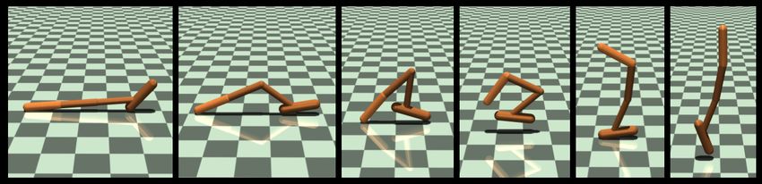
5Figure 2: Hopper completes a get-up sequence before moving to its normal forward walking behavior.
The getup sequence is learned along side the forward hopping in the modified task setting.
Table 3: Modified Task Description
vx is forward velocity; θ is the heading angle; pz is the height of torso; and a is the action.
Task Description Reward (des = desired value)
Agent swims in the desired direction.
Swimmer (3D) vx − 0.1|θ − θdes | − 0.0001||a||2
Should recover (turn) if rotated around.
Agent hops forward as fast as possible. 2 2
Hopper (2D) vx − 3||pz − pdes
z || − 0.1||a||
Should recover (get up) if pushed down.
Agent walks forward as fast as possible. 2 2
Walker (2D) vx − 3||pz − pdes
z || − 0.1||a||
Should recover (get up) if pushed down.
Agent moves in the desired direction. 2 2
Ant (3D) vx − 3||pz − pdes
z || − 0.01||a||
Should recover (turn) if rotated around.
3. Changes to environment’s physics parameters, such as mass and joint torque. If the agent has
sufficient power, most tasks are easily solved. By reducing an agent’s action ability and/or
increasing its mass, the agent is more under-actuated. These changes also produce more realistic
looking motion.
Combined, these modifications require that the learned policies not only make progress towards
maximizing the reward, but also recover from adverse conditions and resist perturbations. An example
of this is illustrated in Figure 4, where the hopper executes a get-up sequence before hopping to
make forward progress. Furthermore, at test time, a user can interactively apply pushing and rotating
perturbations to better understand the failure modes. We note that these interactive perturbations may
not be the ultimate test for robustness, but a step towards this direction.
(a) (b)
Figure 3: (a) Learning curve on modified walker (diverse initialization) for different policy archi-
tectures. The curves are averaged over three runs with different random seeds. (b) Learning curves
when using different number of conjugate gradient iterations to compute F̂θ−1
k
g in (5). A policy with
300 Fourier features has been used to generate these results.
6Figure 4: We test policy robustness by measuring distanced traveled in the swimmer, walker, and
hopper tasks for three training configurations: (a) with termination conditions; (b) no termination,
and peaked initial state distribution; and (c) with diverse initialization. Swimmer does not have a
termination option, so we consider only two configurations. For the case of swimmer, the perturbation
is changing the heading angle between −π/2.0 and π/2.0, and in the case of walker and hopper, an
external force for 0.5 seconds along its axis of movement. All agents are initialized with the same
positions and velocities.
Representational capacity The supplementary video demonstrates the trained policies. We con-
centrate on the results of the walker task in the main paper. Figure 3 studies the performance as
we vary the representational capacity. Increasing the Fourier features allows for more expressive
policies and consequently allow for achieving a higher score. The policy with 500 Fourier features
performs the best, followed by the fully connected neural network. The linear policy also makes
forward progress and can get up from the ground, but is unable to learn as efficient a walking gait.
Perturbation resistance Next, we test the robustness of our policies by perturbing the system with
an external force. This external force represents an unforeseen change which the agent has to resist
or overcome, thus enabling us to understand push and fall recoveries. Fall recoveries of the trained
policies are demonstrated in the supplementary video. In these tasks, perturbations are not applied to
the system during the training phase. Thus, the ability to generalize and resist perturbations come
entirely out of the states visited by the agent during training. Figure 4 indicates that the RBF policy
is more robust, and also that diverse initializations are important to obtain the best results. This
indicates that careful design of initial state distributions are crucial for generalization, and to enable
the agent to learn a wide range of skills.
5 Summary and Discussion
The experiments in this paper were aimed at trying to understand the effects of (a) representation; (b)
task modeling; and (c) optimization. We summarize the results with regard to each aforementioned
factor and discuss their implications.
Representation The finding that linear and RBF policies can be trained to solve a variety of
continuous control tasks is very surprising. Recently, a number of algorithms have been shown to suc-
cessfully solve these tasks [3, 28, 4, 14], but all of these works use multi-layer neural networks. This
suggests a widespread belief that expressive function approximators are needed to capture intricate
details necessary for movements like running. The results in this work conclusively demonstrates that
this is not the case, at least for the limited set of popular testbeds. This raises an interesting question:
what are the capability limits of shallow policy architectures? The linear policies were not exemplary
7in the “global” versions of the tasks, but it must be noted that they were not terrible either. The RBF
policy using random Fourier features was able to successfully solve the modified tasks producing
global policies, suggesting that we do not yet have a sense of its limits.
Modeling When using RL methods to solve practical problems, the world provides us with neither
the initial state distribution nor the reward. Both of these must be designed by the researcher and
must be treated as assumptions about the world or prescriptions about the required behavior. The
quality of assumptions will invariably affect the quality of solutions, and thus care must be taken in
this process. Here, we show that starting the system from a narrow initial state distribution produces
elaborate behaviors, but the trained policies are very brittle to perturbations. Using a more diverse
state distribution, in these cases, is sufficient to train robust policies.
Optimization In line with the theme of simplicity, we first tried to use REINFORCE [20], which
we found to be very sensitive to hyperparameter choices, especially step-size. There are a class of
policy gradient methods which use pre-conditioning to help navigate the warped parameter space of
probability distributions and for step size selection. Most variants of pre-conditioned policy gradient
methods have been reported to achieve state of the art performance, all performing about the same [19].
We feel that the used natural policy gradient method is the most straightforward pre-conditioned
method. To demonstrate that the pre-conditioning helps, Figure 3 depicts the learning curve for
different number of CG iterations used to compute the update in (5). The curve corresponding to
CG = 0 is the REINFORCE method. As can be seen, pre-conditioning helps with the learning
process. However, there is a trade-off with computation, and hence using an intermediate number of
CG steps like 20 could lead to best results in wall-clock sense for large scale problems.
We chose to compare with neural network policies trained with TRPO, since it has demonstrated
impressive results and is closest to the algorithm used in this work. Are function approximators
linear with respect to free parameters sufficient for other methods is an interesting open question
(in this sense, RBFs are linear but NNs are not). For a large class of methods based on dynamic
programming (including Q-learning, SARSA, approximate policy and value iteration), linear function
approximation has guaranteed convergence and error bounds, while non-linear function approximation
is known to diverge in many cases [29, 30, 31, 32]. It may of course be possible to avoid divergence
in specific applications, or at least slow it down long enough, for example via target networks or
replay buffers. Nevertheless, guaranteed convergence has clear advantages. Similar to recent work
using policy gradient methods, recent work using dynamic programming methods have adopted
multi-layer networks without careful side-by-side comparisons to simpler architectures. Could a
global quadratic approximation to the optimal value function (which is linear in the set of quadratic
features) be sufficient to solve most of the continuous control tasks currently studied in RL? Given
that quadratic value functions correspond to linear policies, and good linear policies exist as shown
here, this might make for interesting future work.
6 Conclusion
In this work, we demonstrated that very simple policy parameterizations can be used to solve many
benchmark continuous control tasks. Furthermore, there is no significant loss in performance due to
the use of such simple parameterizations. We also proposed global variants of many widely studied
tasks, which requires the learned policies to be competent for a much larger set of states, and found
that simple representations are sufficient in these cases as well. These empirical results along with
Occam’s razor suggests that complex policy architectures should not be a default choice unless side-
by-side comparisons with simpler alternatives suggest otherwise. Such comparisons are unfortunately
not widely pursued. The results presented in this work directly highlight the need for simplicity
and generalization in RL. We hope that this work would encourage future work analyzing various
architectures and associated trade-offs like computation time, robustness, and sample complexity.
Acknowledgements
This work was supported in part by the NSF. The authors would like to thank Vikash Kumar, Igor
Mordatch, John Schulman, and Sergey Levine for valuable discussion.
8References
[1] Volodymyr Mnih et al. Human-level control through deep reinforcement learning. Nature, 518,
2015.
[2] David Silver et al. Mastering the game of go with deep neural networks and tree search. Nature,
529, 2016.
[3] John Schulman, Sergey Levine, Philipp Moritz, Michael Jordan, and Pieter Abbeel. Trust region
policy optimization. In ICML, 2015.
[4] Timothy P Lillicrap, Jonathan J Hunt, Alexander Pritzel, Nicolas Heess, Tom Erez, Yuval Tassa,
David Silver, and Daan Wierstra. Continuous control with deep reinforcement learning. In
ICLR, 2016.
[5] Yuval Tassa, Tom Erez, and Emanuel Todorov. Synthesis and stabilization of complex behaviors
through online trajectory optimization. IROS, 2012.
[6] Igor Mordatch, Emanuel Todorov, and Zoran Popovic. Discovery of complex behaviors through
contact-invariant optimization. ACM SIGGRAPH, 2012.
[7] Mazen Al Borno, Martin de Lasa, and Aaron Hertzmann. Trajectory Optimization for Full-
Body Movements with Complex Contacts. IEEE Transactions on Visualization and Computer
Graphics, 2013.
[8] Sergey Levine, Chelsea Finn, Trevor Darrell, and Pieter Abbeel. End-to-end training of deep
visuomotor policies. JMLR, 17(39):1–40, 2016.
[9] Vikash Kumar, Emanuel Todorov, and Sergey Levine. Optimal control with learned local
models: Application to dexterous manipulation. In ICRA, 2016.
[10] Vikash Kumar, Abhishek Gupta, Emanuel Todorov, and Sergey Levine. Learning dexterous
manipulation policies from experience and imitation. CoRR, abs/1611.05095, 2016.
[11] Lerrel Pinto and Abhinav Gupta. Supersizing self-supervision: Learning to grasp from 50k tries
and 700 robot hours. In ICRA, 2016.
[12] Greg Brockman, Vicki Cheung, Ludwig Pettersson, Jonas Schneider, John Schulman, Jie Tang,
and Wojciech Zaremba. Openai gym, 2016.
[13] John Schulman, Philipp Moritz, Sergey Levine, Michael Jordan, and Pieter Abbeel. High-
dimensional continuous control using generalized advantage estimation. In ICLR, 2016.
[14] Shixiang Gu, Timothy Lillicrap, Zoubin Ghahramani, Richard E. Turner, and Sergey Levine.
Q-Prop: Sample-Efficient Policy Gradient with An Off-Policy Critic. In ICLR, 2017.
[15] Igor Mordatch, Kendall Lowrey, and Emanuel Todorov. Ensemble-CIO: Full-body dynamic
motion planning that transfers to physical humanoids. In IROS, 2015.
[16] Aravind Rajeswaran, Sarvjeet Ghotra, Balaraman Ravindran, and Sergey Levine. EPOpt:
Learning Robust Neural Network Policies Using Model Ensembles. In ICLR, 2017.
[17] Fereshteh Sadeghi and Sergey Levine. (CAD)2RL: Real Single-Image Flight without a Single
Real Image. In RSS, 2016.
[18] Josh Tobin, Rachel Fong, Alex Ray, Jonas Schneider, Wojciech Zaremba, and Pieter Abbeel.
Domain randomization for transferring deep neural networks from simulation to the real world.
In IROS, 2017.
[19] Yan Duan, Xi Chen, Rein Houthooft, John Schulman, and Pieter Abbeel. Benchmarking deep
reinforcement learning for continuous control. In ICML, 2016.
[20] Ronald J. Williams. Simple statistical gradient-following algorithms for connectionist reinforce-
ment learning. Machine Learning, 8(3):229–256, 1992.
9[21] Shun-ichi Amari. Natural gradient works efficiently in learning. Neural Computation, 10:251–
276, 1998.
[22] Sham M Kakade. A natural policy gradient. In NIPS, 2001.
[23] Jan Peters. Machine learning of motor skills for robotics. PhD Dissertation, University of
Southern California, 2007.
[24] Ali Rahimi and Benjamin Recht. Random Features for Large-Scale Kernel Machines. In NIPS,
2007.
[25] Emanuel Todorov, Tom Erez, and Yuval Tassa. MuJoCo: A physics engine for model-based
control. In International Conference on Intelligent Robots and Systems, 2012.
[26] Tom Erez, Yuval Tassa, and Emanuel Todorov. Infinite-horizon model predictive control for
periodic tasks with contacts. In RSS, 2011.
[27] Tom Erez, Kendall Lowrey, Yuval Tassa, Vikash Kumar, Svetoslav Kolev, and Emanuel Todorov.
An integrated system for real-time model predictive control of humanoid robots. In Humanoids,
2013.
[28] Nicolas Heess, Gregory Wayne, David Silver, Tim Lillicrap, Tom Erez, and Yuval Tassa.
Learning continuous control policies by stochastic value gradients. In NIPS, 2015.
[29] Alborz Geramifard, Thomas J Walsh, Stefanie Tellex, Girish Chowdhary, Nicholas Roy, and
Jonathan P How. A tutorial on linear function approximators for dynamic programming and
reinforcement learning. Foundations and Trends R in Machine Learning, 6(4):375–451, 2013.
[30] Jennie Si. Handbook of learning and approximate dynamic programming, volume 2. John
Wiley & Sons, 2004.
[31] Dimitri P Bertsekas. Approximate dynamic programming. 2008.
[32] Leemon Baird. Residual algorithms: Reinforcement learning with function approximation. In
ICML, 1995.
10A Choice of Step Size
An important design choice in the version of NPG presented in this work is normalized vs un-
normalized step size. The normalized step size corresponds to solving the optimization problem in
equation (3), and leads to the following update rule:
s
δ
θk+1 = θk + F̂θ−1 g.
g F̂θ−1
T
k
g k
On the other hand, an un-normalized step size corresponds to the update rule:
θk+1 = θk + α F̂θ−1
k
g.
The principal difference between the update rules correspond to the units of the learning rate
parameters α and δ. In accordance with general first order optimization methods, α scales inversely
with the reward (note that F does not have the units of reward). This makes the choice of α highly
problem specific, and we find that it is hard to tune. Furthermore, we observed that the same values
of α cannot be used throughout the learning phase, and requires re-scaling. Though this is common
practice in supervised learning, where the learning rate is reduced after some number of epochs, it
is hard to employ a similar approach in RL. Often, large steps can destroy a reasonable policy, and
recovering from such mistakes is extremely hard in RL since the variance of a gradient estimate for a
poorly performing policy is higher. Employing the normalized step size was found to be more robust.
These results are illustrated in Figure 5
Swimmer: α vs δ Hopper: α vs δ Walker: α vs δ
1000
200
2000
0
Return
Return
Return
0 α=0.01 α=0.01 -1000 α=0.01
α=0.05 α=0.05 α=0.05
α=0.1 α=0.1 α=0.1
α=0.25 0 α=0.25 α=0.25
-2000
α=1.0 α=1.0 α=1.0
-200 α=2.0 α=2.0 α=2.0
δ=0.01 δ=0.01 δ=0.01
δ=0.05 δ=0.05 -3000 δ=0.05
δ=0.1 δ=0.1 δ=0.1
-400 -2000 -4000
10 20 30 40 50 20 40 60 80 50 100 150 200 250
Training Iterations Training Iterations Training Iterations
Figure 5: Learning curves using normalized and un-normalized step size rules for the diverse versions
of swimmer, hopper, and walker tasks. We observe that the same normalized step size (δ) works
across multiple problems. However, the un-normalized step size values that are optimal for one task
do not work for other tasks. In fact, they often lead to divergence in the learning process. We replace
the learning curves with flat lines in cases where we observed divergence, such as α = 0.25 in case
of walker. This suggests that normalized step size rule is more robust, with the same learning rate
parameter working across multiple tasks.
B Effect of GAE
For the purpose of advantage estimation, we use the GAE [13] procedure in this work. GAE uses
an exponential average of temporal difference errors to reduce the variance of policy gradients at
the expense of bias. Since the paper explores the theme of simplicity, a pertinent question is how
well GAE performs when compared to more straightforward alternatives like using a pure temporal
difference error, and pure Monte Carlo estimates. The λ parameter in GAE allows for an interpolation
between these two extremes. In our experiments, summarized in Figure 6, we observe that reducing
variance even at the cost of a small bias (λ = 0.97) provides for fast learning in the initial stages.
This is consistent with the findings in Schulman et al. [13] and also make intuitive sense. Initially,
when the policy is very far from the correct answer, even if the movement direction is not along the
gradient (biased), it is beneficial to make consistent progress and not bounce around due to high
11variance. Thus, high bias estimates of the policy gradient, corresponding to smaller λ values make
fast initial progress. However, after this initial phase, it is important to follow an unbiased gradient,
and consequently the low-bias variants corresponding to larger λ values show better asymptotic
performance. Even without the use of GAE (i.e. λ = 1), we observe good asymptotic performance.
But with GAE, it is possible to get faster initial learning due to reasons discussed above.
Walker: GAE
0
Return
-2500
GAE=0.00
GAE=0.50
GAE=0.90
-5000 GAE=0.95
GAE=0.97
GAE=1.00
50 100 150 200 250
Training Iterations
Figure 6: Learning curves corresponding to different choices of λ in GAE. The experiment is
performed on the diverse/interactive walker task described in this paper. λ = 0 corresponds to
a high bias but low variance version of policy gradient corresponding to a TD error estimate:
Â(st , at ) = rt + γV (st+1 ) − V (st ); while λ = 1 corresponds to a low bias but high variance
PT 0
Monte Carlo estimate: Â(st , at ) = t0 =t γ t −t rt0 − V (st ). We observe that low bias is important
to achieve best performance asymptotically, but a low variance gradient can help in the initial stages.
12You can also read