TROPICAL CYCLONE INTENSITY ESTIMATIONS OVER THE INDIAN OCEAN USING MACHINE LEARNING
←
→
Page content transcription
If your browser does not render page correctly, please read the page content below
T ROPICAL CYCLONE INTENSITY ESTIMATIONS OVER THE
                                                             I NDIAN OCEAN USING M ACHINE L EARNING

                                                                  Koushik Biswas                                         Sandeep Kumar
                                                    Department of Computer Science, IIIT Delhi             Department of Computer Science, IIIT Delhi
arXiv:2107.05573v1 [physics.ao-ph] 7 Jul 2021

                                                           New Delhi, India, 110020.                                          &
                                                            koushikb@iiitd.ac.in                                  Department of Mathematics,
                                                                                                        Shaheed Bhagat Singh College, University of Delhi
                                                                                                                   New Delhi, India, 110020.
                                                                                                    sandeepk@iiitd.ac.in, sandeep_kumar@sbs.du.ac.in

                                                                                             Ashish Kumar Pandey
                                                                                       Department of Mathematics, IIIT Delhi
                                                                                            New Delhi, India, 110020.
                                                                                         ashish.pandey@iiitd.ac.in

                                                                                                    July 15, 2021

                                                                                                    A BSTRACT
                                                         Tropical cyclones are one of the most powerful and destructive natural phenomena on earth. Tropical
                                                         storms and heavy rains can cause floods, which lead to human lives and economic loss. Devastating
                                                         winds accompanying cyclones heavily affect not only the coastal regions, even distant areas. Our
                                                         study focuses on the intensity estimation, particularly cyclone grade and maximum sustained surface
                                                         wind speed (MSWS) of a tropical cyclone over the North Indian Ocean. We use various machine
                                                         learning algorithms to estimate cyclone grade and MSWS. We have used the basin of origin, date,
                                                         time, latitude, longitude, estimated central pressure, and pressure drop as attributes of our models.
                                                         We use multi-class classification models for the categorical outcome variable, cyclone grade, and
                                                         regression models for MSWS as it is a continuous variable. Using the best track data of 28 years over
                                                         the North Indian Ocean, we estimate grade with an accuracy of 88% and MSWS with a root mean
                                                         square error (RMSE) of 2.3. For higher grade categories (5-7), accuracy improves to an average of
                                                         98.84%. We tested our model with two recent tropical cyclones in the North Indian Ocean, Vayu and
                                                         Fani. For grade, we obtained an accuracy of 93.22% and 95.23% respectively, while for MSWS, we
                                                         obtained RMSE of 2.2 and 3.4 and R2 of 0.99 and 0.99, respectively.

                                                Keywords Machine Learning · Tropical Cyclone · Cyclone intensity · Maximum sustained surface wind speed

                                                1    Introduction

                                                Tropical cyclones are rapidly rotating storm systems centered in a low-pressure region. Tropical cyclones cause heavy
                                                rain, strong wind, large storm surges near landfall, and tornadoes, which results in loss of property and lives. About
                                                1.9 million people have died because of tropical cyclones worldwide during the last two centuries [1, 2]. The North
                                                Indian ocean (which includes the Bay of Bengal and Arabian sea) alone has seen some of the most devastating tropical
                                                cyclones. In 2019, both coasts of India experienced substantial damages because of Vayu and Fani.
                                                It is of high importance to estimate the intensity of a tropical cyclone. A standard indicator of the intensity of the
                                                storm is the maximum sustained surface wind speed (MSWS). The World Meteorological Organization categorizes
                                                the low-pressure systems using the ranges of MSWS of the tropical cyclones [3]. The categorization can be used to
                                                determine possible storm surges and damage impact on land [4].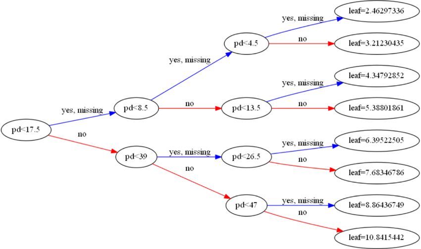
Tropical cyclone intensity estimations over the Indian ocean using Machine Learning

In most tropical cyclone basins, satellite-based Dvorak technique or reconnaissance air-crafts are used to estimate
MSWS [5]. These techniques provide reasonable estimates but require advanced machinery. Therefore, estimating
MSWS from other tropical cyclone parameters is a significant problem. Much work has been done towards this problem;
see [6, 7] and references therein for a complete history of the work relating to cyclone intensity prediction.
We propose a method to estimate MSWS based on other characteristics of a tropical cyclone like date, time, latitude,
longitude, pressure drop and estimated central pressure. We use machine learning algorithms to devise a regression
model to estimate MSWS from other characteristics. We further employ machine learning classification algorithms to
predict the grade of the cyclone based on these characteristics.

2     Materials and methods

2.1   Data

The best track dataset of tropical cyclonic disturbances are collected from the Regional Specialized Meteorological Cen-
tre, New Delhi (http://www.rsmcnewdelhi.imd.gov.in/index.php?option=com_content&view=article&
id=48&Itemid=194&lang=en) has been used in this study for the period from 1990 to 2017 in the North Indian ocean.
The basin of origin, name (if there any), date and time of occurrence, position (latitude and longitude), Class number
(or T No.), estimated central pressure, MSWS, pressure drop, grade, outermost closed isobar and diameter of outermost
closed isobar of tropical cyclones are provided in the dataset. We define terms which we are going to use in the analysis
below [3]:

       • Basin of origin(BOO): The Arabian sea, Bay of Bengal, or land is the possible basin of origins of any cyclone.
       • Date and Time: The date and time of the origin of the cyclone.
       • Latitude and Longitude: The latitude and longitude in degrees along the path of the cyclone.
       • Estimated central pressure (ECP): It is the surface pressure at the center of the tropical cyclone as measured
         or estimated (in hPa (hectopascals)).
       • Pressure drop (PD): It is the drop in the pressure with respect to the atmospheric pressure. It is also measured
         in hPa.
       • Maximum sustained surface wind (MSWS): The maximum sustained surface wind speed is the highest
         average of 3 minutes surface wind speed occurring within the circulation of the system. It is measured in knots
         (nautical miles per hour), which is the same as 1.86 Kilometers per hour.
       • Grade: Any tropical cyclone that develops within the North Indian Ocean between 100◦ E and 45◦ E is
         monitored by the India Meteorological Department (IMD). Tropical cyclone intensity scale according to
         cyclone category are given in the following table:

                         Grade            Low pressure system               MSWS (in knots)
                           1             Low Pressure Area (LP)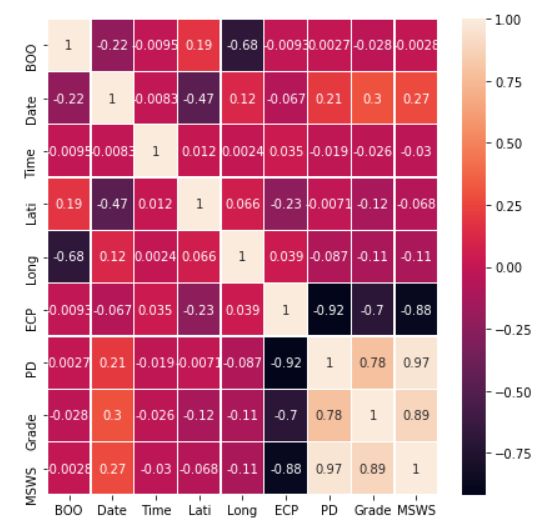
Tropical cyclone intensity estimations over the Indian ocean using Machine Learning
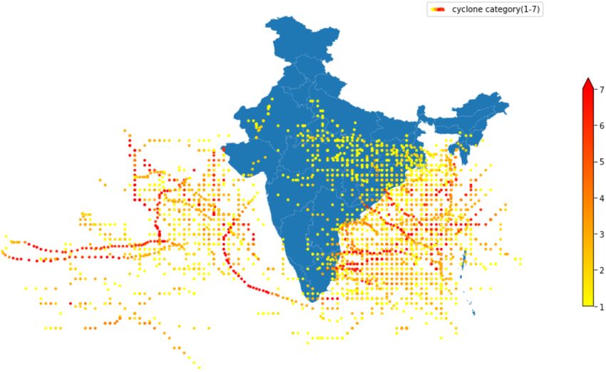
Figure 1: Cyclones hitting India since 1990-2017.
Characteristics Subdivisions Number of data points
Arabian Sea 1149
Basin of Origin Bay of Bengal 2707
Land 165
Pre-Monsoon (March - May) 791
Season Monsoon (June to September) 1208
Post-monsoon (October - February) 2022
1 1433
2 915
3 920
Grade 4 266
5 15
6 205
7 267
Table 2: Baseline Data.
2.2 Methodology
The MSWS is a continuous variable, while the grade is a categorical variable. Therefore, we use various machine
learning regression and classification algorithms (XGBoost, Gradient Boosting Machine, Linear Regression, Decision
Tree, Random Forest, SVM, Naive Bayes, Logistic Regression) for the prediction of MSWS and grade. In what follows,
we briefly describe these algorithms.
2.2.1 Decision tree
Decision Tree [8] is one of the most popular supervised machine learning algorithms used for both classification and
regression techniques. The algorithm can be represented by an inverted tree with a root node at the top and other nodes
connected to it through branches. Each node corresponds to a feature and a value assigned to the feature, while each
branch represents a decision taken for the output variable based on the node it is emanating. To decide which feature to
be placed at a node, we use measures like the Gini index, Entropy, or Information gain. For a given attribute X,
• Entropy is defined as X
E(X) = −P (X = x) log2 (X = x),
• Information gain is defined as
IG(X, x) = E(X) − E(X|x),
3Tropical cyclone intensity estimations over the Indian ocean using Machine Learning
• Gini index is defined as X
1− (P (X = x))2
where P denotes the probability, E(X) denotes the entropy and E(X|x) is the conditional entropy for a particular
instance x of X. We can determine the importance of a given attribute of a feature vector by calculating one of the
above for that attribute.
2.2.2 Random Forest
Random forest [9] is an ensemble learning method that can be used for both classification and regression. It generates
multiple decision trees as part of the training process and outputs the mode (average) of these trees as per the
classification (regression) problem. This approach solves the problem of overfitting, which is prevalent in the case of
Decision Trees.
2.2.3 Gradient Boosting Machine
Gradient Boosting Machine [10] is an ensemble machine learning technique that is used for both classification and
regression problems. It depends on the boosting technique where each weak learner is assigned a large weight to convert
them to a strong learner in an iterative manner.
2.2.4 XGBoost
XGBoost [11] is one of the most popular recent supervised learning tree boosting scalable machine learning algorithms,
which is based on function approximation and several regularization techniques. It is used for both classification and
regression problems. Let ybi is the outcome from the ensemble model defined as follows:
K
X
ybi = φ(xi ) = fk (xi ), fk ∈ F
k=1
where F = {f (x) = wq(x) }, q : Rm → T , w ∈ RT is the space of all regression trees and T denotes the total number
of leaves in the tree. In the above equation, fk represents a regression tree and fk (xi ) is the outcome given by the kth
tree to the ith entries in the data. The goal in XGBoost is to minimize the following regularized objective function:
n
X K
X
L(φ) = l(yi , ybi ) + Ω(fk )
i=1 k=1
where l is the loss function. To avoid high complexity of the model, a regularization term Ω is used which is given by
T
1 1 X 2
Ω(fk ) = γT + λ||w||2 = γT + λ w
2 2 j=1 j
Where γ and λ are regularization parameters, the best split at any given node can be found from the following formula:
G2L G2R (GL + GR )2
1
Lsplit = + − −γ
2 HL + λ HR + λ HL + HR + λ
Where L stands for left-hand node and R stands for right-hand node by letting I = IL ∪ IR . Figure 3 shows the
XGBoost tree for the estimation of MSWS.
2.2.5 Linear Regression
In Linear Regression [12], a hyperplane is estimated that gives best linear relationship between independent variables
(features) and dependent variable (target). The prediction model (hypothesis) is given by :
hθ (X) = θ0 + θ1 x1 + θ2 x2 + · · · + θn xn
where X = (x1 , x2 , . . . , xn ) represents the input vector and θ = (θ0 , θ1 , θ2 , . . . , θn ) are the coefficients that determine
the hyperplane. These coefficients are learned through an iterative process called gradient descent by minimizing the
following loss function:
Xm
J(θ) = (hθ (Xi ) − yi )2 ,
i=1
where Xi denotes the ith input vector and yi corresponding target value.
4Tropical cyclone intensity estimations over the Indian ocean using Machine Learning
2.2.6 Logistic Regression
Logistic regression [13] is a classifier that can be used to solve a multiclass prediction problem. Its an extension of
Linear Regression, where the classification problem is converted into regression problem by estimating the log(odds)
of each class inPplace of probability itself. If pi denotes the probability of ith class then the log(odds) for this class is
defined as pi / j6=i pj .
2.2.7 Support Vector Machines (SVM)
SVM [14] can be used for both classification and regression problems. Like the Linear regression, SVM tries to find a
separating hyperplane, but with maximum margin. The learning problem is converted into an objective (nonlinear)
maximization problem, subject to linear constraints. Using the tools of Linear Programming Problem (LPP), few input
vectors (called support vectors) are selected that can be used for prediction. The nonlinear separating case of input
vectors can be handled with kernels techniques.
2.2.8 Naive Bayes
Naive Bayes [15] can be used for both classification and regression problems. The Naive Bayes algorithm is based on
Bayes’ theorem with an assumption that the features are linearly independent. Suppose X1 , X2 , · · · , Xn are real-valued
attributes, and Y is the set of all possible outcomes. Now according to the Bayes’ theorem,
P (Y = yi )P (X1 , X2 , · · · , Xn |Y = yi )
P (Y = yi |X1 , X2 , · · · , Xn ) = P .
k P (Y = yk )P (X1 , X2 , · · · , Xn |Y = yk )
If we assume that Xi are conditionally independent for given outcome set Y , then the above equation can be written as
Q
P (Y = yi ) j P (Xj |Y = yi )
P (Y = yi |X1 , X2 , · · · , Xn ) = P Q
k P (Y = yk ) j P (Xj |Y = yk )
The above equation is used for the classification problem. Similarly, we can define Naive Bayes for regression problems,
where the sum in the above equation will be replaced by integration.
2.2.9 Metrics
To evaluate the performance of regression models for MSWS, we use the Root Mean square error (RMSE) and
Coefficient of determination (R2 ).
• RMSE: If there are m sample points with yi as actual value and ybi as predicted value evaluated from the
model, then RMSE is defined as
v
u m
u1 X
t (yi − ybi )2 .
m i=1
RMSE is always non-negative and should be close to 0.
• R2 : The coefficient of determination (R2 ) is defined as
SEŷ
R2 = 1 −
SEȳ
Pm
where total sum ofPsquares, SEȳ , is defined as SEȳ = i=1 (yi − y¯i )2 andPresidual sum of squares, SEŷ is
m 1 m
defined as SEŷ = i=1 (yi − ybi )2 . Here, ȳ is the mean of the data, ȳ = m i=1 yi .
The confusion matrix is used to determine the performance of the classification model on the test data. For classification
models, multi-class classification accuracy has been measured using the confusion matrix [16]. Accuracy is the ratio
between all correctly predicted samples to all possible samples.
correctly predicted samples
Accuracy =
total number of test samples
5Tropical cyclone intensity estimations over the Indian ocean using Machine Learning
Figure 2: Correlation between variables.
3 Results and Discussions
3.1 Correlation analysis
The correlation matrix of all variables is given in Figure 2. The grade is weakly correlated with all the variables except
ECP and PD. Also, the correlation of grade with ECP is negative, suggesting that if central pressure is low, the intensity
of the cyclone is high. The MSWS shares a similar correlation with ECP as the grade. This is not surprising as grade
is directly evaluated from MSWS; see Table 1. PD has a strong positive correlation with MSWS. A linear regression
suggests the following relationship between MSWS and PD
MSWS ≈ 1.6 PD +22.3
in the North Indian Ocean. Notice that in [17], a similar relationship between MSWS and PD (MSWS ≈ 1.176PD + 30)
was reported for tropical cyclones in Central North Pacific Ocean.
3.2 Model selection and validation
We use 10-fold cross-validation for each of the models. In each fold, we split the data into training and validation
sets in the ratio of 4:1. Then, each ML algorithm is applied to the training set to train the model. At every step, the
performances (RMSE, R2 , or accuracy) of the model are recorded, and the average of each of these performances is
reported in Tables 3a and 3b.
It is evident from Table 3a that XGBoost is outperforming other models with an RMSE of 2.3 and R2 of 0.99. Notice
from Table 1 that the range of values of MSWS for a particular grade is always greater than or equal to 5, and since
XGBoost is predicting MSWS with an RMSE of 2.3, we expect that XGBoost will also predict grade with very high
accuracy. That is definitely the case, as from Table 3b, XGboost has an accuracy of 87.15% in predicting the grade.
However, the Decision Tree with Entropy of depth 4 outperforms XGBoost in predicting the grade with an accuracy of
87.91%.
Moreover, if we fix the classification model for the grade to be the Decision Tree with Entropy of depth 4, Table 4
represents the accuracy in predicting a particular category for the grade. The model predicts the top three high-intensity
categories (SCS, VSCS, and SS) of grade with an average accuracy of 98.84%.
6Tropical cyclone intensity estimations over the Indian ocean using Machine Learning
Model Accuracy
Model RMSE R2
XGBoost 87.15
XGBoost 2.30 .99
GBM 85.73
Gradient Boosting
2.80 0.97 Decision Tree
Machine 87.91
Entropy(Depth-4)
Decision Tree 3.91 0.94 84.76
Gini(Depth-4)
Random Forest 3.12 0.96
Random forest 85.95
Linear Regression 5.07 0.92
Naive Bayes 86.39
SVM
Logistic 71.28
Kernel:-RBF 6.11 0.90
SVM
Kernel:Linear 5.69 0.91
Kernel:-RBF 78.48
Kernel: Polynomial 3.93 0.95
Kernel: Linear 86.90
(4th-degree)
Kernel: Polynomial 84.36
Naive Bayes 3.38 0.97
(degree 4)
(a) Regression Analysis on MSWS.
(b) Classification(Multi-class) Analysis on Cyclone grade.
Category Accuracy
LP 98.33
D 77.92
DD 78.37
CS 88.72
SCS 100
VSCS 99.51
SS 97
Table 4: Classification accuracy of different Cyclone Grade.
Figure 3: XGBoost tree for MSWS.
3.3 Testing on Vayu and Fani
We test our model on two recent tropical cyclones, Vayu and Fani. Vayu was a grade 7 tropical cyclone which hit the
Indian west coast in June 2019. Around 6.6 million people were affected in northwestern India by the cyclone [18].
Fani was also a grade 7 tropical cyclone that hit the Indian state of Odisha in April-May 2019. Due to Fani, India and
7Tropical cyclone intensity estimations over the Indian ocean using Machine Learning
Figure 4: Scatter plot of actual and model-predicted MSWS for Fani and Vayu.
Figure 5: Actual and model predicted grade along track of Fani.
Bangladesh faced heavy damages. At least 89 people have been reported died, and damages caused estimated around
US$8.1 billion [19].
We checked the performance of the best model to predict MSWS, XGBoost, on Vayu and Fani. The RMSE is 2.2 and
3.4, while R2 is 0.99 and 0.99 for Vayu and Fani, respectively. Figure 4 depicts the actual values of MSWS and values
predicted by the XGBoost model during the course of Vayu and Fani.
The best model to predict grade, Decision Tree with Entropy with depth 4, predicts different grades during the course of
Vayu and Fani with an accuracy of 93.22% and 95.23%, respectively. The actual and predicted grades along the track of
Vayu and Fani is shown in Figures 5 and 6.
8Tropical cyclone intensity estimations over the Indian ocean using Machine Learning
Figure 6: Actual and model predicted grade along track of Vayu.
4 Conclusion
Estimating the intensity of tropical cyclones on a real-time basis is a problem worth studying, considering the human
life and economic loss involved. In this study, we explored various machine learning techniques and reported their
performance to estimate the Maximum Surface Sustained Wind Speed and intensity of the tropical cyclone. Our
research finds that the ML model XGBoost and Decision Tree can be used for the estimation of MSWS and intensity
with excellent performance over the North Indian ocean.
Acknowledgement
Authors are thankful to the Indian Meteorological Department (IMD) for providing the data archives.
Conflict of Interest
All the authors declare that they have no conflict of interest.
References
[1] RF Adler. Estimating the benefit of tropical tropical cyclone data in saving lives. 2005.
[2] SK Rautaray, P Panigrahi, and PK Panda. Tropical Cyclone and Crop Management Strategies. 2014.
[3] National Weather Service. Tropical cyclone names and definitions. 2018.
[4] V K Victor. The Role of Remote Sensing in Predicting and Determining Coastal Storm Impacts. Journal of
Coastal Research, 2009(256):1264 – 1275, 2009.
[5] D Thompson. How are hurricane wind speeds determined? 2016.
[6] S Chaudhuri, D Dutta, S Goswami, and A Middey. Intensity forecast of tropical cyclones over north indian ocean
using multilayer perceptron model: skill and performance verification. Natural Hazards, pages 97–113, 2012.
[7] Q Li, Z Li, Y Peng, Y Wang, L Li, H Lan, S Feng, L Sun, G Li, and X Wei. Statistical regression scheme for
intensity prediction of tropical cyclones in the northwestern pacific. American Meteorological Society, 2018.
[8] JR Quinlan. Induction of decision trees. Mach. Learn., 1(1):81–106, March 1986.
[9] L Breiman. Random forests. Mach. Learn., 45(1):5–32, October 2001.
[10] JH Friedman. Greedy function approximation: A gradient boosting machine. Annals of Statistics, 29:1189–1232,
2000.
[11] T Chen and C Guestrin. Xgboost: A scalable tree boosting system. CoRR, abs/1603.02754, 2016.
9Tropical cyclone intensity estimations over the Indian ocean using Machine Learning
[12] JM Stanton. Galton, pearson, and the peas: A brief history of linear regression for statistics instructors. Journal of
Statistics Education, 9(3):null, 2001.
[13] SH Walker and DB Duncan. Estimation of the probability of an event as a function of several independent
variables. Biometrika, 54(1-2):167–179, 06 1967.
[14] C Cortes and V Vapnik. Support-vector networks. In Machine Learning, pages 273–297, 1995.
[15] I Rish. An empirical study of the naive bayes classifier. Technical report, 2001.
[16] C Manliguez. Generalized confusion matrix for multiple classes, 11 2016.
[17] HE Rosendal and SL Shaw. Relationship of maximum sustained winds to minimum sea level pressure in central
north pacific tropical cyclones. Noaa technical memorandum nwstm, 1982.
[18] RSMC, India meteorological department. Very severe cyclonic storm “vayu” over southeast & adjoining eastcentral
arabian sea and lakshadweep (10 june – 17 june, 2019): Summary. 2019.
[19] UNICEF. Cyclone fani situation report. 2019.
10You can also read