An implementation of Artificial Neural Reservoir Computing Technique for Inflow Forecasting of Nagarjuna Sagar dam
←
→
Page content transcription
If your browser does not render page correctly, please read the page content below
International Journal of Recent Technology and Engineering (IJRTE)
ISSN: 2277-3878, Volume-8, Issue-1, May 2019
An implementation of Artificial Neural Reservoir
Computing Technique for Inflow Forecasting of
Nagarjuna Sagar dam
B.Pradeepakumari, Kota.Srinivasu
Abstract:All over India flash flood or recurring flood is one of It is due to the fact that training is limited only to the output
the major natural disaster causing life and economic threats. layer all other layers need not be trained [9]. A reservoir is a
Several times a year, some or the other state disaster dynamic system capable of modeling complex patterns in a
management in India have to face this. Forecasting system for time series input sequence. Artificial Neural Network
inflow of any dam plays a key role in this disaster and its
(ANN) model is successful in various fields forpredictions.
recovery. Current forecasting systems follow conventional,
graphical metrological procedures and limited Artificial Neural Even in hydrological predictions it has shown success but
Network models.This work provides novel model for forecasting with few limitations in cases of non-stationary data[10,11].
inflow of a dam. Proposed model uses Neural Reservoir A non-stationary time series data has a variable variance and
Computing for forecasting inflow. Forecasts are based on mean that does not remain constant or same to their long –
standard dam parameters like inflow. Most importantly, forecasts run mean over time. On the other hand, stationary time
done are several days ahead of time. This would help disaster series data reverts around a constant long-term mean
management systems to be prepared well in advance to save lives. exhibits a constant variance independent of time.Daily flow
Proposed system is demonstrated over data from two major dams time series data are often nonlinear and non-stationary [12].
in Andhra Pradesh. Results are compared with statistical
Non stationary behavior of a time series is due to variations
forecasting models like AR, MA, & ARIMA and Artificial Neural
Networks (ANN) model. Comparison prove proposed neural in seasons and trends. This significantly affects
reservoir computing model to be better than existing systems. predictability of classical models for forecasting. Various
researchers have applied hybrid models of neural networks
Keywords: Artificial Neural Reservoir Computing; ARIMA; or complex pre-processing or their combinations to improve
Inflow forecasting; Nagarjunasagar dam; prediction performance with limited success.Now, Reservoir
computing has emerged as an effective tool to simplify the
I. INTRODUCTION non-stationary in the dataset and has been widely applied by
coupling with neural networks for rainfall runoff modeling.
Water inflow is major factor driving any dam dynamics. Reservoir computing has shown its steady performance on
Knowledge about near future inflow amount enables time series forecasting problems of various domains like
effective and efficient dam operations and management. It wind power, finance, weather [12, 13].
also enables flood forecasting, drought control, irrigation
management, hydropower generation and effective daily II. STUDY AREA
usage. So, an accurate model for forecasting inflow values is
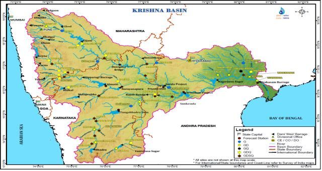
necessary. Classical rainfall and runoff models exist, such as Nagarjuna sagar dam catchment, a part of the Krishna river
empirical, conceptual, physically, and data-driven [1,2]. basin extends over Andhra Pradesh, maharastra and
Promising results are obtained using Data-driven models in Karnataka having the total area 2,58,948 sq.km which is
different fields of water resources with [3,4,5]. At the same nearly 8% of the total geographical area of India. The area
time, researchers have realized complex nature of lies between 73°17' to 81°09' east longitudes and 13°10' to
relationship between rainfall and runoff so various complex 19°22' north latitude with an elevation 1337 meters above
models are introduced like fuzzy logic [6], support vector mean sea level.The catchment falls within sub tropical
regression [7], and artificial neural networks (NNs) [2]. climate, and daily mean relative humidity varies from 17 to
Human decision making model is inspiration behind current 92% with alternating dry and wet periods.The total length of
neural network models. Neural networks have been widely the river from origin to it’s out fall into bay of Bengal is
applied as an effective method for modeling highly 1400 km.
nonlinear phenomenon in hydrological processes [8].
Reservoir computing is an improved artificial intelligence
paradigm that requires significantly less computations than
existing ANN models for training the datasets.
Revised Manuscript Received on May 18, 2019
B. Pradeeepakumari, Dept. of Civil Engg., Acharya Nagarjuna
University, Guntur, India.
K. Srinivasu, Dept. of Civil Engg., RVR&JC College of Engnn.,
Guntur, India.
Published By:
Blue Eyes Intelligence Engineering
Retrieval Number A9287058119/19©BEIESP 860 & Sciences Publication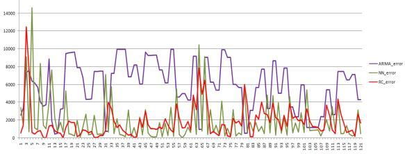
An implementation of Artificial Neural Reservoir Computing Technique for Inflow Forecasting of
                                          Nagarjuna Sagar dam
There are two major canals from this dam one going to right            Figure 3 and 4 shows exploratory data analysis of inflow
and other to left side. Comparison of these two canals for             data collected. Fig 3ashows pattern of monthly average for
various parameters is presented using figure 2. Here length            all fifteen year inflow data. Clearly,August is having highest
of the main canal is described in unit (102 km), max bed               peak followed by September or October peaks. Minimum
width is in unit (10mt), depth of flow is in unit (mt), max            peaks are observed in May and June.Other figure, fig 3b
discharge is in unit of (102 cum/s), head regulator still level        shows great peaks in 2005, 2006 and 2009 highlighting
unit is (102 mt), length of branches and channels is in unit           floods in Andhra Pradesh. Figure 4a makes it clear that
(103 km), and finally localized ayacut is measured in unit             floods occurred in August for 2005 and 2006 but in
(lakh ha). Both canals have strength in different parameters.          November for 2009. Another highlight of this analysis is,
                                                                       2003, 2012 and 2015 were least inflow years in Nagarjuana
                                                                       Sagar dam.

     Fig 2. Canal Statistics for Nagarjuna Sagar Dam
Additionally,the study area comprises with agricultural land
accounting to 75.86% of total area and 4.07% covered by
water bodies. Krishna catchment consists of 7 reservoirs
namely konya,Tungabhadra, srisailam, nagajunasagar,                                  Fig 3: Average Inflow a) per month
almatti, narayanapur , Bhadra with intention of hydropower
generation ,water supply for irrigation, industrial and
domestic uses and flood control.
Data set used in the study
Daily inflow data is collected for 15 years (from 2003-
2017). Data has an entry of inflow record per day for all
these years. Missing values and extreme values are treated
with standard procedures. After this basic processing,data is
used for forecasting. Sample inflow values for Nagarjuana
Sagar Dam are shown in Table 1. Table 2 shows statistics
for inflow data of same dam.It is very clear that in past this
dam has received very high inflow of more than 1 million in                           Fig 3: Average Inflowb) per year
a single day.
  Date      Inflow        Date    Inflow      Date          Inflow
01-01-                   11-01-
             8921                 3174     21-01-2017       12620
2017                      2017
02-01-                   12-01-
             6511                 5425     22-01-2017       10116
2017                      2017
03-01-                   13-01-
             5333                 2849     23-01-2017       8276
2017                      2017
04-01-                   14-01-
             12415                3784     24-01-2017       7365
2017                      2017
05-01-                   15-01-
             17363                 36      25-01-2017       2220
2017                      2017
06-01-                   16-01-
             15662                1992     26-01-2017       2261
2017                      2017
07-01-
             13307
                         17-01-
                                  7606     27-01-2017        790
                                                                           Fig 4: Inflow graph for every year a) between 2003 to
2017                      2017                                                                      2010
08-01-                   18-01-
             20849                6972     28-01-2017       1908
2017                      2017
09-01-                   19-01-
             2600                 11986    29-01-2017       2172
2017                      2017
10-01-                   20-01-
             6388                 13621    30-01-2017       4355
2017                      2017
 Table 1: Sample Data of Inflow values from Nagarjuna
                     Sagar Dam
                                  Nagarjuana Sagar
         Mean                                 21585.08925
         Mode                                           0
                                                                            Fig 4: Inflow graph for every year b) 2011 to 2017
         Median                                      5016
         Standard Deviation                   64210.37905
         Minimum                                        0
         Maximum                                 1173690
  Table 2: Statistical Details of Nagarjuna Sagar Dam
         inflow Data for 15 years (2003-2017)

                                                                             Published By:
                                                                             Blue Eyes Intelligence Engineering
     Retrieval Number A9287058119/19©BEIESP                          861     & Sciences Publication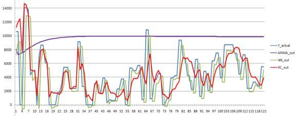
International Journal of Recent Technology and Engineering (IJRTE)
                                                                              ISSN: 2277-3878, Volume-8, Issue-1, May 2019

    III.       DAM INFLOW MONITORING                        FOR                 ARIMA(p,d,q) = f(AR(p), I(d), MA(q)) - eq(3)
               FLOOD FORECASTING
                                                                       2. Artificial Neural Network Based Methods
    1.     Statistical Methods:
                                                                       In recent times Artificial Neural Network (ANN) based
     Traditionally statistical methods are used for forecasting        models are flooding various application domains. In field of
in various domains. Domains like flood predictions, finance,           forecasting also, they have achieved enormous
share market, soil quality, and predictive maintenance are             results[10].Here, multiple layers of neurons doprocess input,
just some examples for their application. Models like                  extract features with various weights, and finally leading to
ARIMA, AR, and MA are popularly used statistical models.               output. These networks can be modeled for numeric forecast
Also, models like Halts winter, spline interpolation, and              or categorical forecast as well.
regression analysis are used regularly.                                In application field of non stationary time series forecasting,
                                                                       normal ANN architectures are not efficient.Special
    a.     Auto Regression (AR):                                       architecture of ANN called reservoir computing has proved
                                                                       significant than other models here[11].
This is one of the classical statistical techniques for time
series predictions. Here variable to be predicted is related                1. Reservoir Computing in ANN
with its own history. This model assumes a linear relation             It is a dynamic system modeling based on reservoir of
between historical values and current value of the input               neurons. Here, there are three major components, namely
variable.This relation is used for future value prediction for         input layer, output layer and set of neurons called
the variable. A particular variable may be related to itself for       reservoir.An example of reservoir computing neural network
multiple historical values. So, auto regression is performed           architecture is shown in figure 1. Input and output layer are
for previous ‘p’ values. It can be stated in details for               as per the standard neural network definition [15].
equation 1.
          AR(x, p) =f( x-1 , x-2 , … , x-p) - eq (1)

Here, equation 1 depicts the current value ‘x’ is dependent
on its ‘p’ historical values, x-1 , x-2 , … , x-p. Function ‘f’ is
linear function which detects the statistical pattern of
historical values and maps it to current value.This model
may suffer from non-stationary issues.
This model is being applied in various domains like finance,
flood routing, predictive maintenance and Medicare.
Another variant of this model is used in medical domain.
Here auto-regression is applied varying with time. General
additive method is combined with auto regression for better                Fig 5: Architecture of Reservoir Computing Neural
results, especially in psychological dynamics[14].                                                     Network
                                                                       Input is directly given to input layer. Input can vary in size
b.        Moving Average (MA)                                          and number of variables. In time series forecasting generally
A simple modification of averaging technique for time                  there are two types, single variable time series and
series analysis is known as moving average or simple                   multivariate time series. In addition, same input with along
moving average. In time series absolute mean or average                with its several historical instances can act as input. So input
value over all samples is not very relevant as data keeps on           I can be defined as,
changing with time [14]. To find relevant patterns in current                            I = (i0, i-1, i-2, … i-p) … eq (4)
data, moving average is taken.                                                    Here, Iis set of input values with its ‘p’ historical
Here, a fixed window of size ‘q’ is used. All values in this           instances. For example, ‘i0’ is current instance of input and
window are averaged. This window keeps on sliding one                  ‘i-1’ is historical instance of one unit time.
step at a time. So, at each time‘t’, there is a separate window        Output layer provides numeric output for time series
and moving average value.                                              forecasting problems. This number is treated as output
                                                                       forecast valueof inflow ‘Inpred’. In training phase, if there is
                           MA(x,q) =               -eq(2)              differencein actual inflow ‘Inactual’ and predictedinflow
                                                                       ‘Inpred’, then erroris back propagated only to output layer.
c.     Auto Regression            Integration    and    Moving         Error can be calculated using Mean Absolute Error (eq 5) or
Average (ARIMA)                                                        Mean Squared Error (eq 6) or Root Mean Squared Error
                                                                       formula as given by eq 7. Mean Absoluter Percentage Error
This is one of the most powerful statistical models used in            (MAPE) is another popular error major for time series
forecasting. It comprises of three parts, Auto Regression              analysis. It is given in eq 8. Here in following equations ‘n’
(AR), Moving Average (MA) and Integration (I).AR & MA                  is number of total predicted samples.
components are as discussed earlier. Another part,
Integration,works by differencing provided series to
itself.Degree of differencing is represented by ‘d’ value.             MAE =
Such differencing helps in better pattern modeling. So,                           … eq (5)
together all these three parts can handle even very complex
time series models.

                                                                           Published By:
                                                                           Blue Eyes Intelligence Engineering
      Retrieval Number A9287058119/19©BEIESP                     862       & Sciences Publication
An implementation of Artificial Neural Reservoir Computing Technique for Inflow Forecasting of
                                               Nagarjuna Sagar dam
                MSE =                          … eq (6)

              RMSE =                               … eq (7)

             MAPE =                                 … eq (8)

          2. Concept of Neural Reservoir
     A Reservoir is network of neurons which are sparsely
     connected to each other. Also, there can beself loops                Fig 6. Approach for Implementing Reservoir Computing
     amongst themselves. Neuron based reservoir is unaffected                                     Model
     and is not modified on back propagation of error[15]. Only
     input and output layers get affected by error back                              IV.       RESULTS AND DISCUSSION
     propagation. So, there is no problem of vanishing gradient
     here. Also, such architecture of reservoir represents dynamic      Experiment is conducted to compare various methods for
     system. Another limitation is, at each neuron only limited         inflow forecasting. For this purpose Nagarjuna Sagar Dam
     modification to the input is possible. Difference between          data is used. Data is taken from project management system,
     Output and Input of a neuron in reservoir is between 0 and         Government of Andhra pradesh, India website [17,18,19].
     1. This limitation reduces the gradient explosion problem          Here proposed Reservoir Computing (RC) method is
     [16].                                                              compared with statistical method ARIMA and Artificial
     Let ‘ Ir’ be input to a neuron in reservoir and ‘ Or ’ be output   Neural Networks (ANN). Each model is made to forecast on
     from that neuron. Then relation between input and output is        test data. Figure 7 shows the predicted values graph of
     given by equation                                                  ARIMA, ANN and RC along with actual values for those
             || Or – Ir || ≤ δ … where 0 ≤ δ ≤ 1 … eq (9)               days. Predictions of ARIMA can be concluded to be general
                                                                        predictions. It predicts a pattern that inflow will be
                                                                        consistently increasing. But it clearly fails to catch pattern in
3.     Approach for Implementing Reservoir Computing                    future inflow values. Another prediction curve is of ANN,
       Model                                                            which seems to follow the inflow pattern. But after careful
     Here, reservoir computing model is proposed for inflow             observation it is very clear that ANN is following the pattern
     forecasting. So, first input and output layers are defined.        and not predicting it. So, for example in case there is change
     Number of neurons in input layer depends on number of              in pattern on day 30 then it will change its pattern for day
     inputs. Here past six values of inflow are taken as input to       31. And same thing continues for the entire predicted
     predict inflow. On the other hand output layer has only            pattern. This clearly indicates model is poor to lead the
     single neuron as this is a regression task. Next, capacity of      predictions. Additionally it has missed the major peaks in
     reservoir in terms of ‘x’ number of neurons is set. Also, ‘δ’      predictions leading to large errors. On other hand proposed
     is defined for better performance of the reservoir.                reservoir computing model has captured the pattern of
     Sl. No        Type of Dataset          Date Range                  inflow time series. It has presented a dynamic predictions
                                                  01/01/2003 to         and it’s not just following the inflow pattern. Reservoir
         1            Training Dataset          01/09/2017 (5357        computing predictions have better captured the peaks
                                                    samples)            leading to less error.
                                                  02/09/2017 to
         2              Test Dataset            31/12/2017 (121
                                                    samples)

             Table 3. Training and Testing Dataset Details

               In training phase input of all training samples is
     provided. Then model is trained using one of the error
                                                                          Fig 7: Result comparison for ARIMA, ANN and Reservoir
     MAE, MSE or RSME. Error is back-propagated only to the
                                                                                                 Computing
     output and input layer. Output layer, also known as read out
     layer, weights are adjusted to give best output. Training is
     carried out in multiple epochs on the same data. Training
     and testing dataset details are given in table 3. Next, for
     testing the performance predictions are made on testing data.
     On these predictions MAE, MSE and RMSE is calculated to
     check optimal performance of the model. For further
     optimization of the model, reservoir parameters like number
     of neurons ‘x’ or ‘δ’ are adjusted. Then training is done             Fig 8: AbsoluteError curve comparison for ARIMA,
     again and further optimized model is obtained.                                  ANN and Reservoir Computing

                                                                             Published By:
                                                                             Blue Eyes Intelligence Engineering
          Retrieval Number A9287058119/19©BEIESP                    863      & Sciences Publication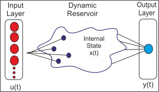
International Journal of Recent Technology and Engineering (IJRTE)
                                                                                  ISSN: 2277-3878, Volume-8, Issue-1, May 2019

Figure 8 presents absolute error curve comparison between                         neural network for flood forecasting. Neural ComputAppl 23(1):231–
                                                                                  246
ARIMA, ANN and RC. ARIMA has high error nearly for all
                                                                            7.    Herrera M, Torgo L, Izquierdo J, Perez-Garcıa R (2010) Predictive
the samples. ANN has major error when it has missed the                           models for forecasting hourlyurban water demand. J Hydrol 387(1–
peaks.Finally, proposed reservoir computing model has                             2):141–150
missed some peaks but at many places it has achieved                        8.    Abrahart RJ, Anctil F, Coulibaly P, Dawson CW, Mount NJ, See LM,
                                                                                  Shamseldin AY,
reasonable predictions.                                                     9.    Coulibaly, P. (2010). Reservoir computing approach to Great Lakes
                         ARIMA            ANN             RC                      water level forecasting. Journal of hydrology, 381(1-2), 76-88.
       MAE                                                                  10.   Cannas B, Fanni A, See L, Sias G (2006) Data pre-processing for
                          41.95           14.14          10.5                     river flow forecasting using neural networks: wavelet transforms and
      (10^3)
                                                                                  data partitioning. Phy Chem Earth 31(18):1164–1171
     MSE (10^8)           50.72            6.63          6.24               11.   Partal T (2009) Modeling evapotranspiration using discrete wavelet
      RMSE                                                                        transform and neuralnetworks. Hydrol Process 23(25):3545–3555
                           6.79            2.45          2.38               12.   Wang, J., Niu, T., Lu, H., Yang, W., & Du, P. (2019). A Novel
      (10^3)
                                                                                  Framework of Reservoir Computing for Deterministic and
      MAPE                111.66           24.7          11.18                    Probabilistic Wind Power Forecasting. IEEE Transactions on
 Table 4: Statistical Comparison of Inflow Predictions                            Sustainable Energy.
                                                                            13.   Wyffels, F., &Schrauwen, B. (2010). A comparative study of
Table 4 clearly demonstrates better performance of                                reservoir computing strategies for monthly time series prediction.
Reservoir computing over ANN and ARIMA over MAE,                                  Neurocomputing, 73(10-12), 1958-1964.
MSE, RMSE and MAPE.                                                         14.   Yamamoto, T. (1981), Predictions of multivariate autoregressive-
                                                                                  moving average models. Biometrika, 68(2), 485-492.
                                                                            15.   Steil, J. J. (2004, July). Backpropagation-decorrelation: online
                    V.        CONCLUSION                                          recurrent learning with O (N) complexity. In 2004 IEEE International
                                                                                  Joint Conference on Neural Networks (IEEE Cat. No. 04CH37541)
Flood forecasting is an important task in India for disaster                      (Vol. 2, pp. 843-848). IEEE.
                                                                            16.   Gallicchio, C., Micheli, A., &Pedrelli, L. (2017). Deep reservoir
management. Here a neural reservoir computing approach is                         computing: A critical experimental analysis. Neurocomputing, 268,
presented for flood forecasting using inflow prediction. This                     87-99.
method has given promising results over other existing                      17.   National Water Development Agency of India, www.nwda.gov.in
methods.                                                                    18.   Water Resources Information System of India , www.india-
                                                                                  wris.nrsc.gov.in
Here in this work, flood forecasting task is done using
Nagarjuna Sagar Dam inflow Data for 15 years (2003-
2017).Data analysis shows dynamic patterns in inflow data.
Existing inflow forecasting methods ARIMA             and
ANN have limitation to handle such non-stationary time
series data. Proposed neural reservoir computing method has
captured the pattern well and has given minimal error in
predictions. These models are evaluated based on Mean
Absolute Error, Mean Squared Error, Root Mean Squared
Error and Mean Absolute Percentage Error measures. On all
measures proposed neural reservoir computing method is
proved to be better than other existing models.
Results depicted to potential of Artificial neural reservoir
computing in forecasting task. So, this model can be further
applied on various civil domains like predictive maintenance
of reservoirs, seepage forecasting in Earthen Dams and soil
moisture level prediction.

REFERENCES

1.   Verma AK, Jha MK, Mahana RK (2010) Evaluation of HEC-HMS
     and WEPP for simulating watershed runoff using remote sensing and
     geographical information system. Paddy WaterEnviron 8(2):131–144
2.   Adamowski JF (2008) Peak daily water demand forecast modelling
     using artificial neural networks. Water ResourPlann Manage
     134(2):119–128
3.   Mukerji A, Chatterjee C, Raghuwanshi NS (2009) Flood forecasting
     using ANN, neuro-fuzzy, andneuro-GA models. J HydrolEng
     14(6):647–652
4.   Tiwari MK, Chatterjee C (2010) Development of an accurate and
     reliable hourly flood forecastingmodel using wavelet-bootstrap-ANN
     hybrid approach. J Hydrol 394:458–470
5.   Tiwari MK, Chatterjee C (2011) A new wavelet-bootstrap-ANN
     hybrid model for daily dischargeforecasting. J Hydroinf 13(3):500–
     519
6.   Kant A, Suman PK, Giri BK, Tiwari MK, Chatterjee C, Nayak PC,
     Kumar S (2013) Comparisonof multi-objective evolutionary neural
     network, adaptive neuro-fuzzy inference system andbootstrap-based

                                                                                  Published By:
                                                                                  Blue Eyes Intelligence Engineering
       Retrieval Number A9287058119/19©BEIESP                         864         & Sciences Publication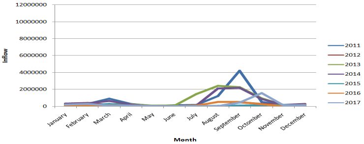
You can also read