Generalized Joint Probability Density Function Formulation in Turbulent Combustion using DeepONet
←
→
Page content transcription
If your browser does not render page correctly, please read the page content below
Sub Topic: Turbulent Combustion

                                                                               12th U.S. National Combustion Meeting
                                                                  Organized by the Central States Section of the Combustion Institute
                                                                                     May 24–26, 2019 (Virtual)
                                                                                        College Station, Texas

                                                   Generalized Joint Probability Density Function Formulation in
                                                             Turbulent Combustion using DeepONet
arXiv:2104.01996v1 [physics.flu-dyn] 5 Apr 2021

                                                                  Rishikesh Ranade1 , Kevin Gitushi2 , and Tarek Echekki2, *
                                                                                1 CTO Office, Ansys Inc, Canonsburg, PA, US
                                                            2 Mechanical     Engineering, North Carolina State University, Raleigh, NC, US
                                                                               * Corresponding author: techekk@ncsu.edu

                                                         Abstract: Joint probability density function (PDF)-based models in turbulent combustion provide
                                                         direct closure for turbulence-chemistry interactions. The joint PDFs capture the turbulent flame dy-
                                                         namics at different spatial locations and hence it is crucial to represent them accurately. The joint
                                                         PDFs are parameterized on the unconditional means of thermo-chemical state variables, which can
                                                         be high dimensional. Thus, accurate construction of joint PDFs at various spatial locations may
                                                         require an exorbitant amount of data. In a previous work, we introduced a framework that alleviated
                                                         data requirements by constructing joint PDFs in a lower dimensional space using principal compo-
                                                         nent analysis (PCA) in conjunction with Kernel Density Estimation (KDE). However, constructing
                                                         the principal component (PC) joint PDFs is still computationally expensive as they are required to
                                                         be calculated at each spatial location in the turbulent flame. In this work, we propose the concept
                                                         of a generalized joint PDF model using the Deep Operator Network (DeepONet). The DeepONet
                                                         is a machine learning model that is parameterized on the unconditional means of PCs at a given
                                                         spatial location and discrete PC coordinates and predicts the joint probability density value for the
                                                         corresponding PC coordinate. We demonstrate the accuracy and generalizability of the DeepONet
                                                         on the Sandia flames, D, E and F. The DeepONet is trained based on the PC joint PDFs observed in
                                                         flame E and yields excellent predictions of joint PDFs shapes at different spatial locations of flames
                                                         D and F, which are not seen during training.
                                                         Keywords: Turbulent combustion, Joint PDF, Machine Learning, DeepONet

                                                  1. Introduction

                                                  Modeling closure for turbulence-chemistry interactions presents an important challenge in turbu-
                                                  lent combustion modeling [1]. Joint probability density function (PDFs) based approaches are
                                                  commonly used to determine a direct closure for the turbulence-chemistry interactions in the gov-
                                                  erning equations and accelerate high fidelity simulations. Most turbulence-chemistry closure ap-
                                                  proaches fall under two categories, Flamelet-based and PDF-based [2]. The Flamelet approaches
                                                  rely on the assumption of the PDF shape (e.g. β -PDF) and hence, the resulting closure models
                                                  are limited to certain combustion modes and regimes. On the other hand, the PDF approaches
                                                  calculate the joint PDF distributions. Although these methods are computationally costly, but they
                                                  provide an accurate representation of the closure terms.
                                                      In turbulent combustion simulations, the thermo-chemical space is high dimensional and this
                                                  presents difficulties in the construction of joint PDFs. Hence, closure approaches for turbulent
                                                  flames rely on effectively representing the thermo-chemical state in a lower dimensional set of

                                                                                                           1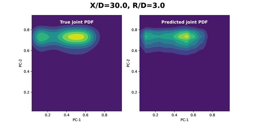
Sub Topic: Turbulent Combustion

variables. In many approaches, the lower-dimensional basis is established using physical vari-
ables, such as mixture fraction, progress variable, scalar dissipation etc., that efficient describe the
turbulent flames. With the developments in machine learning and statistical methods, recent ap-
proaches have relied on available simulation or experimental data to extract a lower-dimensional
basis from the thermo-chemical state using methods such as, Principal Component Analysis (PCA)
[3]. PCA determines a low-dimensional basis for the data, such that the leading PCs represent the
maximum explained variance in the data. In the context of turbulent combustion, PCA provides a
linear projection to represent the entire thermo-chemical state by a significantly smaller set of pa-
rameters, known as principal components (PCs). PCA has been used in combustion for chemistry
reduction (see for example Vajda et al. [4] ) as well as for the parameterization of the composition
space [5–14].
    The effective parameterization of the thermo-chemical state is an important first step in the
computation of joint PDFs. As stated above, the Flamelet-based approaches presume a joint PDF
shape in this lower dimensional manifold but PDF-based approaches rely on computation of the
joint PDF. In the PDF-based approaches the joint PDF is computed mainly by PDF transport or by
using data generated from lower-dimensional simulations, such as LEMLES [15] and the LESODT
[16]. In these approaches, the turbulent flame is modeled stochastically on 1-D domains using the
linear eddy model (LEM) [17] and the one-dimensional turbulence (ODT) model [18]. The scalar
statistics collected at each spatio-temporal location are then used to calculate joint PDFs, which
may be used to accelerate the full fidelity simulations. Recently, Ranade and Echekki [13, 14]
introduced a novel turbulence-chemistry closure framework that used instantaneous experimental
measurements to construct joint PDFs in a lower dimensional principal component (PC) manifold.
The joint PC PDFs were subsequently used to determine the Favre means of thermo-chemical
scalars and the PC source terms. In this work, the thermo-chemical parameterization was carried
out using principal component analysis (PCA) [3], while the joint PDFs were computed using
kernel density estimation (KDE) [19].
    Kernel density estimation (KDE) [19] is a statistical method that can be used to construct
arbitrary shapes for a joint PDF given discrete data at a given spatial position. In a KDE, a PDF
can be expressed as a weighted sum of discrete kernel functions, K (e.g. Gaussians) centered at
discrete values of the parameters, say the PCs:
                                                                    !
                                               1 n       φ − φ̂φ i
                                   p φ ; φ̃φ =     ∑K h .                                            (1)
                                               n h i=1

In this expression, φ represents the vector of retained PCs, K is the kernel function, h is the so-
called bandwidth, which controls the smoothing of the approximation, and φ̂i is the ith sample of
φ values out of a total of n samples. Such a distribution can be evaluated at a specific spatial point,
which can be parameterized in terms of an unconditional mean for the PCs, φ̃ . Therefore, different
shapes can be evaluated at different spatial positions.
    However, the KDE construction is very local and needs to be implemented at each spatial
location in the space. Moreover, the computation of joint PDFs using KDE can be costly and
require a large amount of data, as the lower-dimensional space increases in size. Hence, it is
imperative to determine a “generalized” PDF that can be adopted for a wide range of unconditional
means for the PCs or spatial position. In their recent work, de Frahan et al. [20] investigated the
reconstruction of PDFs parameterized with the mixture fraction and the progress variable using

                                                   2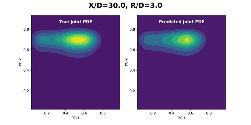
Sub Topic: Turbulent Combustion

three machine learning techniques, random forests, deep learning neural networks and conditional
variational autoencoders. The machine learning techniques showed that the predictions o the joint
PDFs yield improvements on β -function based presumed PDFs using DNS data.
     The most recent work by Lu et al. [21] offers a potentially more powerful strategy to reconstruct
joint PDFs for combustion data. In their approach, Lu et al. [21] have introduced the DeepONet
network, which is designed to learn non-linear operators using sparse training data samples. The
DeepONet networks consist of 2 separate input channels that provide different functional forms of
the learned operators and their instances. The objective of this work is to present a generalizable
model for the joint PDFs using the DeepONet network [21] that can reconstruct joint PDFs at any
given spatial location in a turbulent flame. The main function of the DeepONet is to replace the
KDE-based PDF estimation, as used by Ranade and Echekki [13, 14], and moreover, minimize
the dependence on data requirements to estimate joint PDFs. The generalizable joint PDF model
is trained on Sandia flames E and tested on all the Sandia flames D, E and F at different spatial
locations in the flame. One of the main objectives of this work is to test the generalizability of
the approach to unseen flames and flame conditions. The methodology of learning the PDF using
DeepONet is described in Sec. 2. Next, results are presented and discussed in Sec. 3.

2. Methodology

2.1 PCA parameterization of composition space
As stated earlier, PCA is a technique to linearly transform the vector of thermo-chemical scalars
(e.g. temperature and species mass fractions) to uncorrelated scalars, the PCs:

                                             φ = AT ψ,                                            (2)

where ψ is the vector of N thermo-chemical scalars normalized to yield comparable magnitudes
using maximum and minimum values of these scalars: ψ =(T,Y1 ,Y2 , . . . ,YN−1 ). The PCs vector
φ includes N pc principal components, φ = φ1 , φ2 , . . . , φNpc , which account for a threshold per-
centage of the data variance. For example, the data from the Sandia flames [22] and the Sydney
flames [23–25] require 2 to 3 PCs to capture the entire range of flow conditions and reaction sce-
narios (mixing, extinction and reignition) in these flames. The matrix A includes the leading N pc
eigenvectors of the normalized thermo-chemical scalars covariance matrix.
    The principal components (PCs) serve as a lower dimensional basis which can be used to
compute the joint PDFs and conditional means, that may be used to reconstruct the unconditional
Favre means of thermo-chemical scalars as well as source terms. The unconditional means for the
kth thermo-chemical scalar or its source term can be expressed using the joint thermo-chemical
scalars PDFs as follows:                     Z
                                  ωk (φ ) = hωk |φ i p (φ ) dφ .                                  (3)
                                                φ
                                                Z
                                    ψk (φ ) =       hψ |φ i p (φ ) dφ .                           (4)
                                                φ

In this expression, hωk |φ i is the mean of the thermo-chemical scalars source term and hψ |φ i
is the mean of the thermo-chemical scalars conditioned on the PCs. p (φ ) is the joint PC PDF.
Conditional means are constructed from data; they can be viewed as generalizations of flamelet

                                                     3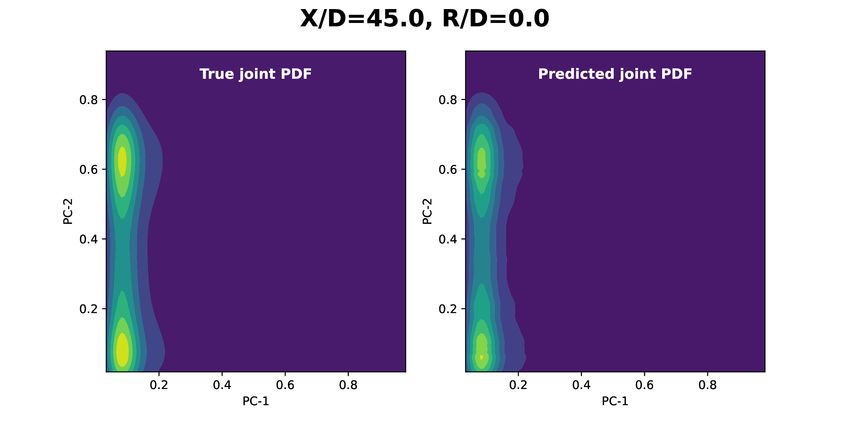
Sub Topic: Turbulent Combustion

libraries or FGMs where the parameterization is based on the PCs instead of prescribed parameters
(e.g. mixture fraction, progress variable).
    It is clear from the formulations in Eqs. 3 and 4 that the accurate estimation of PDF at different
locations in the flame is essential in predicting the means of source terms and thermo-chemical
scalars. Next, we will discuss the DeepONet based joint PDF estimation.

2.2 DeepONet based joint PDF

          Figure 1: Illustration of a DeepONet for determining a PC’s generalized PDF.

    The goal of the DeepONet is to predict a joint probability density function at any spatial loca-
tion in a turbulent flame as a function of the PC state (derived from the thermo-chemical state) at
that location. In the same spirit of general PDFs, the DeepONet ensures that a given PC state is
conditioned with the unconditional mean and variances of PCs at a given location in the turbulent
flame. However, as pointed out in our previous studies [13, 14], the use of the unconditional vari-
ances of PCs is not needed. This observation is primarily associated with the uncorrelated nature
of PCs and the linear relations between thermo-chemical scalars and PCs.
    Although ML-based methods to reconstruct parameterized PDFs have been proposed in the
past [20], the premise of the DeepONet networks is that they are designed to learn operators (in this
case PDF shapes) that can relate prescribed inputs to desired outputs. The DeepONet architecture
that corresponds to the present implementation is illustrated in Fig. 1. It may be observed that the
DeepONet allows for two channels at the input layer in order to accommodate different classes of
inputs. The first input channel corresponds to the unconditional means of PCs at different spatial
locations in the turbulent flame. Conversely, the second input channel is simply the PC state
accessed by the turbulent flame. Both the input channels are passed through 2 fully connected
layers with 64 neurons each. Finally, the outputs of these layers are multiplied element-wise and
the vector sum represents the network output, which in this case is the probability density at a
given PC state conditioned by an unconditional PC mean.

                                                  4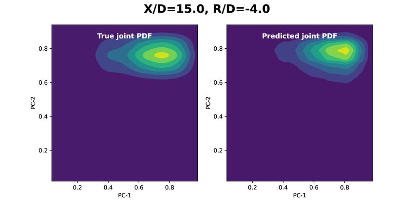
Sub Topic: Turbulent Combustion

2.3 Data generation for training
The data generation process for training the DeepONet is outlined below.

   1. Given instantaneous thermo-chemical data at different spatial locations in the flame, a PCA
      is performed to determine the lower-dimensional PC representation of the instantaneous data
      at all the locations.

   2. Unconditional PC means are determined at each spatial location in the flame.

   3. Gaussian KDE is used to generate the joint PDFs at each spatial locations.

   4. The input data for DeepONet corresponds to the pair of instantaneous PC value and the
      unconditional PC mean at all locations in the flame. Similarly, the output data corresponds
      to the probability density value, determined from pre-computed KDE associated with the
      instantaneous PC conditioned by the unconditional PC mean. For example, if the lower
      dimensional basis is represented by 2 PCs, then each input sample for the DeepONet will
      correspond to (φ1 , φ2 , φ1 , φ2 ) and the output sample will correspond to P(φ1 , φ2 ).

2.4 Training mechanics
The DeepONet network is trained in TensorFlow [26]. Since DeepONets can learn operators from
relatively sparse data sets, a sampling strategy is implemented to maintain the balance of low and
high probabilities in the training set. A mean squared error loss is used to update the network
weights and the training set is split such that 10% is reserved for validation. The training data
covers a sampled range of spatial positions in the turbulent flame; and hence the DeepONet network
represents a generalized joint PDF, which can be recovered at any given point in the flame.

3. Results and Discussion

3.1 Experimental conditions
The dataset used in the following analysis is based on multiscalar measurements in the Sandia
piloted jet flames by Barlow and Frank [22]. The data set consists of 3 flames, D, E and F, charac-
terized by different jet Reynolds numbers. Due to a difference in Reynolds numbers, these flames
exhibit a varying degree of non-equilibrium effects such as flame extinction and reignition. Flame
D has the smallest Reynolds numbers, followed by flame E and flame F. Other details related to
the burner geometry and boundary conditions may be found in Barlow and Frank [22]. The exper-
imental data set corresponding to these flames consists of instantaneous measurements at 70 − 80
axial and radial locations in these flames. The measured species corresponds to T , H2 , O2 , OH,
CH4 , CO, CO2 and H2 O. From a PCA analysis 3 PCs represent 99% of the explained variance
and this is corroborated in a previous work carried out by the authors, [13, 14]. However, in this
work we only retain the first 2 PCs to learn the joint PDFs so as to build a proof of concept for the
DeepONet approach. In future, we may extend this approach to using 3 PCs.
    Since, these flames exhibit a varying degree of non-equilibrium effects the joint PDF shapes
observed at different locations of flame D can be significantly different from flames E and F. As a
result in this work, we use data generated at a handful of spatial locations from flame E for training

                                                  5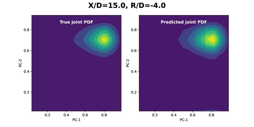
Sub Topic: Turbulent Combustion
the DeepONet and test the generalizability of our approach by predicting joint PDFs on flames D
and flame F.
Figure 2: Comparison of contour plots between DeepONet vs KDE based joint PDFs for Sandia
flame D
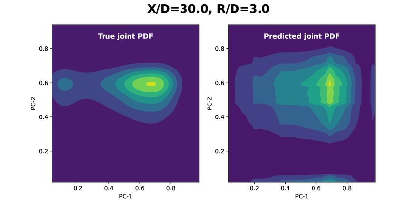
3.2 Contour comparisons
The contour plots of joint PDFs are compared between DeepONet and KDE for the 3 Sandia
flames, D, E and F in Figs. 2, 3 and 4. It may be noted that the DeepONet was only trained on a
6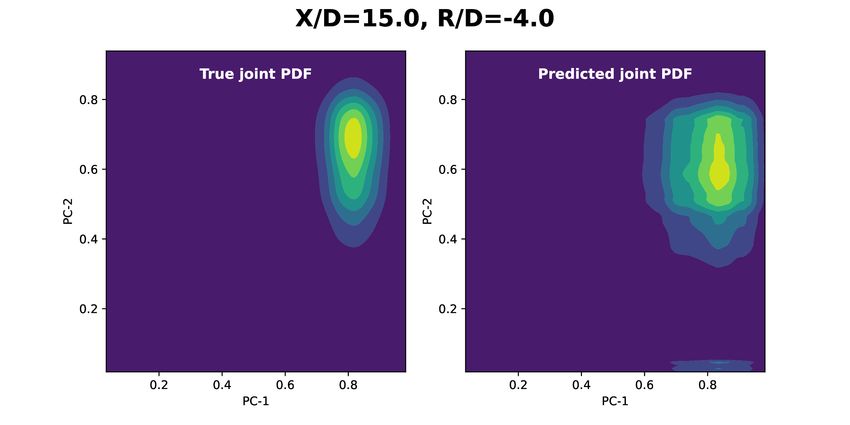
Sub Topic: Turbulent Combustion

few samples from flame E and used for prediction of joint PDFs on all 3 flames. The joint PDFs
are plotted at different axial and radial locations to show the evolution of the flame mixture through
different non-equilibrium effects and that the different locations are characterized by different joint
PDF shapes. These shapes are adequately captured by the DeepONet model that adopts as inputs
their parameterization in terms of the unconditional means for the 2 PCs. Some errors may be
observed in the joint PDFs reconstructed at certain locations of flame F. In future, we will try to
address these errors by including more PCs in the construction of joint PDFs and by conditioning
the DeepONet on the PC variances in addition to the means.

4. Conclusions

The objective of this work was to develop a generalizable model for learning joint PDFs in turbulent
flames using the DeepONet network. The DeepONet based joint PDF approach was demonstrated
on Sandia flames D, E and F, where the network was trained on data from flame E but predictions
of joint PDFs were carried out on all 3 flames. The results show that the DeepONet based recon-
struction approach can reasonably predict the joint PDF shapes for unseen turbulent flames and
flame conditions. The results obtained are very encouraging and more work will be carried out
on addressing inaccuracies and improving the generalizability of the DeepONet based joint PDF
approach.

5. Acknowledgements

This work is supported by the National Science Foundation under grant no. 1941430.

References

 [1] T. Echekki and E. Mastorakos, “Turbulent Combustion Modeling: Advances, New Trends
     and Perspectives”, in: ed. by T. Echekki and E. Mastorako, 1st ed., vol. 95, Springer, Nether-
     land, 2011, chap. Turbulent combustion: Concepts, governing equations and modeling strate-
     gies, p. 392.
 [2] S. Pope, Small scales, many species and the manifold challenges of turbulent combustion,
     Proc. Combust. Inst. 34 (2013) 1–31.
 [3] I. Jolliffe, Principal Component Analysis, 2nd ed., Springer-Verlag New York, 2002.
 [4] S. Vajda, P. Valko, and T. Turányi, Principal component analysis of kinetic models, Int. J.
     Chem. Kin. 17 (2006) 55–81.
 [5] S. Danby and T. Echekki, Proper orthogonal decomposition analysis of autoignition simu-
     lation data of nonhomogeneous hydrogen-air mixtures, Combust. Flame 144 (2006) 126–
     138.
 [6] J. Sutherland and A. Parente, Combustion modeling using principal component analysis,
     Proc. Combust. Inst. 32 (2009) 1563–1570.
 [7] H. Mirgolbabaei and T. Echekki, A novel principal component analysis-based acceleration
     scheme for LES–ODT: An a priori study, Combust. Flame 160 (2013) 898–908.

                                                  7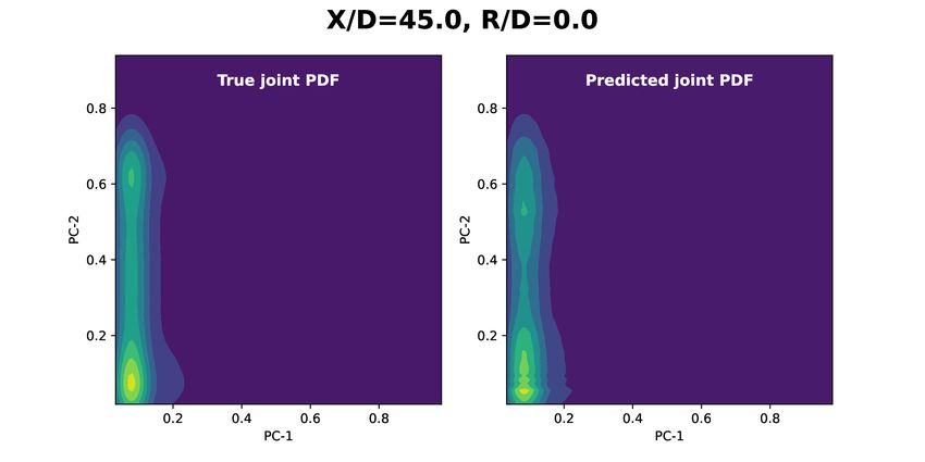
Sub Topic: Turbulent Combustion

Figure 3: Comparison of contour plots between DeepONet vs KDE based joint PDFs for Sandia
flame E

 [8] H. Mirgolbabaei, T. Echekki, and N. Smaoui, A nonlinear principal component analysis
     approach for turbulent combustion composition space, Int. J. Hydrogen Energy 39 (2014)
     4622–4633.
 [9] H. Mirgolbabaei and T. Echekki, Nonlinear reduction of combustion composition space with
     kernel principal component analysis, Combust. Flame 161 (2014) 118–126.

                                             8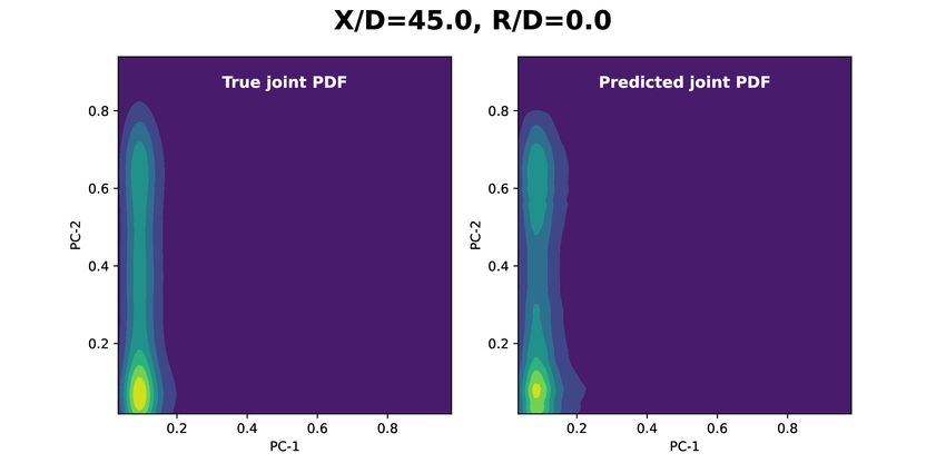
Sub Topic: Turbulent Combustion

Figure 4: Comparison of contour plots between DeepONet vs KDE based joint PDFs for Sandia
flame F

[10] H. Mirgolbabaei and T. Echekki, The reconstruction of thermo-chemical scalars in combus-
     tion from a reduced set of their principal components, Combust. Flame 162 (2015) 1650–
     1652.
[11] T. Echekki and H. Mirgolbabaei, Principal component transport in turbulent combustion: A
     posteriori analysis, Combust. Flame 162 (2015) 1919–1933.

                                             9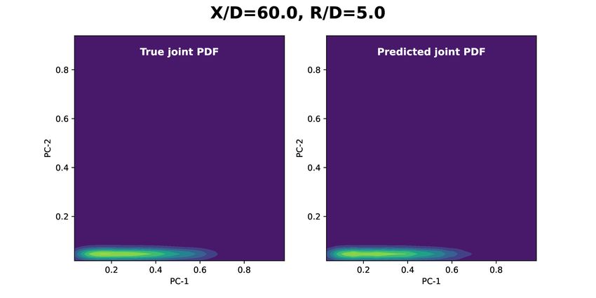
Sub Topic: Turbulent Combustion

[12] O. Owoyele and T. Echekki, Toward computationally efficient combustion DNS with com-
     plex fuels via principal component transport, Combust. Theo. Model. 21 (2017) 770–798.
[13] R. Ranade and T. Echekki, A framework for data-based turbulent combustion closure: A
     priori validation, Combust. Flame 206 (2019) 490–505.
[14] R. Ranade and T. Echekki, A framework for data-based turbulent combustion closure: A
     posteriori validation, Combust. Flame 210 (2019) 279–291.
[15] S. Menon and W. Calhoon, Subgrid mixing and molecular transport modeling for large-eddy
     simulations of turbulent reacting flows, Symp. (Int.) Combust. 26 (1996) 59–66.
[16] S. Cao and T. Echekki, A low-dimensional stochastic closure model for combustion large-
     eddy simulation, J. Turbul. (2008) N2.
[17] A. Kerstein, Linear eddy modeling of turbulent transport. 2. Application to shear layer mix-
     ing, Combust. Flame 75 (1989) 97–413.
[18] A. Kerstein, One-dimensional turbulence: Model formulation and application to homoge-
     neous turbulence, shear flows, and buoyant stratified flows, J. Fluid Mech. 392 (1999) 277–
     334.
[19] A. Bowman and A. Azzalini, Applied smoothing techniques for data analysis: The kernel
     approach with S-Plus illustrations, Oxford University Press, Oxford, Oxford, 1997.
[20] M. de Frahan, S. Yellapantula, R. King, M. Day, and R. Grout, Deep learning for presumed
     probability density function models, Combust. Flame 208 (2019) 436–450.
[21] L. Lu, P. Jin, Z. Zhang, and G. Karniadakis, Learning nonlinear operators with Deep ONnet
     based on the universal approximation theorem of operators, Nature Mach. Intel. 3 (2021)
     218–229.
[22] R. Barlow and J. Frank, Effects of turbulence on species mass fractions in methane/air jet
     flames, Proc. Combust. Inst. 27 (1998) 1087–1095.
[23] S. Meares and A. Masri, A modified piloted burner for stabilizing turbulent flames of inho-
     mogeneous mixtures, Combust. Flame 161 (2014) 484–495.
[24] S. Meares, V. Prasad, G. Magnotti, R. Barlow, and A. Masri, Stabilization of piloted turbu-
     lent flames with inhomogeneous inlets, Proc. Combust. Inst. 35 (2015) 1477–1484.
[25] R. Barlow, S. Meares, G. Magnotti, H. Cutcher, and A. Masri, Local extinction and near-
     field structure in piloted turbulent CH4 /air jet flames with inhomogeneous inlets, Combust.
     Flame 162 (2015) 3516–3540.
[26] M.Abadi, P. Barham, J. Chen, Z. Chen, A. Davis, J. Dean, M. Devin, S. Ghemawat, G.
     Irving, M. Isard, M. Kudlur, J. Levenberg, R.Monga, S. Moore, D. Murray, B. Steiner, P.
     Tucker, V. Vasudevan, P. Warden, M. Wicke, Y. Yu, and X. Zheng, TensorFlow: A system
     for large-scale machine learning, 12th USENIX Symposium on Operating Systems Design
     and Implementation (OSDI 16) USENIX, (2016), pp. 256–283.

                                               10
You can also read