Modeling Rare Baseball Events - Are They Memoryless?
←
→
Page content transcription
If your browser does not render page correctly, please read the page content below
Modeling Rare Baseball Events – Are
They Memoryless?
Michael Huber
Muhlenberg College

Andrew Glen
United States Military Academy

Journal of Statistics Education Volume 15, Number 1 (2007),
www.amstat.org/publications/jse/v15n1/datasets.huber.html

Copyright © 2007 by Michael Huber and Andrew Glen, all rights reserved. This text may
be freely shared among individuals, but it may not be republished in any medium without
express written consent from the authors and advance notification of the editor.

Key Words: Anderson-Darling Goodness-of-Fit Test; Exponential Distribution; Hitting
for the Cycle; Memoryless Property; No-Hit Games; Poisson Process; Triple Plays.

Abstract
Three sets of rare baseball events – pitching a no-hit game, hitting for the cycle, and
turning a triple play – offer excellent examples of events whose occurrence may be
modeled as Poisson processes. That is, the time of occurrence of one of these events
doesn’t affect when we see the next occurrence of such. We modeled occurrences of
these three events in Major League Baseball for data from 1901 through 2004 including a
refinement for six commonly accepted baseball eras within this time period. Model
assessment was primarily done using goodness of fit analyses on inter-arrival data.

1. Introduction
On June 29th, 1990, both Fernando Valenzuela of the Los Angeles Dodgers and Dave
Stewart of the Oakland Athletics pitched no-hit games, the first time two pitchers from
different leagues accomplished the rare feat of holding their opponents hitless on the
same day. Even more amazing, in 1938, Johnny Vander Meer of the Cincinnati Reds
pitched two no-hitters in successive starts (on June 10thand June 14th). Babe Herman, an
outfielder with the Brooklyn Robins, is the only player in Major League Baseball history
(since 1901) to hit for the cycle twice in the same season (1931). On July 17th, 1990, the
Minnesota Twins turned two triple plays against the Boston Red Sox in the same game.
Some events in baseball are more rare than others. Three of the more rare feats – pitching
a no-hit game, hitting for the cycle, and turning a triple play – appear to be reasonably
modeled as Poisson processes.

From 1901 through the end of the 2004 season, there were 206 official no-hit games
pitched in the American and National Leagues. According to the The Book of Baseball
Records, there have been 13 “Near No-Hitters” in the Major Leagues from 1901 - 2004
(instances where the no-hitter had been broken up in extra innings), as well as 25
occurences of a pitcher not allowing a hit in an official game that was less than nine
innings. Because these events do not meet the criteria set forth by Major League Baseball
(MLB) as being a “No-Hit Game,” we did not include them in the data. A no-hit game
(commonly known in baseball as a “no-hitter”) refers to a game in which one of the
teams has prevented the other team from getting an official hit during the entire length of
the game, which must be at least 9 innings by the current Major League Baseball
definition. During this time span there were 225 batters who hit for the cycle – batters
who had a single, a double, a triple, and a home run in the same game. In addition, there
were 511 times from 1901 – 2004 in which a team turned a triple play in a game, which
means that a team recorded three outs in an inning during a single at-bat. We only
consider, by the way, regular season games in this article.

Obvious questions arise. First, how often do no-hitters, hitting for the cycle, and triple
plays occur in a regular season? Also, can we model the number of each that we might
expect to see in a season? Finally, do the chances of these events occurring change during
different eras in baseball history?

2. Modeling Rare Events as Poisson Processes
These three rare incidents offer excellent examples of data that might be modeled by
Poisson processes. The Poisson distribution is often used to characterize the occurrence
of events of a particular type over time, area, or space. By definition, a random variable X
is said to have a Poisson distribution if its probability mass function is

for non-negative integers of x and some positive . For us the parameter will be a rate
per unit time. Additionally, if X has a Poisson distribution with parameter , then both
the expected value of X and the variance of X are equal to . If the annual number of no-
hitters, cycles, and triple plays indeed follow Poisson processes, exponential distributions
will model the distributions of times between consecutive occurences. A random variable
T is said to have an exponential distribution if its probability density function is
where > 0. Additionally, if T has an exponential distribution with parameter , then
the expected value of T equals 1/ and the variance of T is equal to 1/ 2. Note, then,
that the mean and standard deviation are equal.

An important distinction of the exponential distribution is its “memoryless” property. It is
well known that the only continuous distribution that models a memoryless process is the
exponential distribution. The memoryless property implies that the time of the last
occurrence of an event does not affect the time to the next occurrence of that event.
Intuitively, we believe this to be at least approximately true of our three baseball events.

As mentioned earlier, from 1901 to 2004, there have been 206 no-hitters, 225 cycles, and
511 triple plays. These data can be readily found at a number of websites (see
References). The most no-hitters pitched in a single season during this time period is
eight, and the fewest is zero. There has been one season in which eight batters have hit
for the cycle, and the fewest number of occurrences in a season is zero. There have been
three seasons in which eleven triple plays have occurred, but only two seasons in which
no triple play occurred.

Figure 1, Figure 2, and Figure 3 show the total number of occurrences for no-hitters,
cycles, and triple plays per year, respectively, for 1901 – 2004. All three events have a
high number of years when only one, two, or three events occured. Instances where more
than three of each event occurred in a particular season were infrequent, especially in the
no-hitter and cycles data sets (see Table 1). The mean number of no-hitters per year is
= 1.98, or just about two no-hitters per season. The mean number of cycles over this
period is = 2.16, and the mean for the number of triple plays over this period is =
4.91. Even though this last number is higher than for no-hitters or cycles, we will still
consider triple plays to be rare events. To further indicate the rarity of these events, we
note that from 1901 to 2004 there were 159,650 official games played. Consequently,
roughly 0.13% of games were no-hitters, roughly 0.14% of games had a batter hit for the
cycle, and roughly 0.32% of games had a triple play.
Figure 1

Figure 1. Number of No-Hit Games by Year (1901 – 2004).
Figure 2

Figure 2. Number of Cycles by Year (1901 – 2004).
Figure 3

            Figure 3. Number of Triple Plays by Year (1901 – 2004).

Table 1. Actual (versus Estimated) Counts of Rare Events Per Season (1901-2004)
               Count No Hitters Hit for Cycle Triple Plays

                 0      18 (14.3)      18 (12.0)      2 (0.8)

                 1      30 (28.4)      27 (25.9)      6 (3.8)

                 2      21 (28.1)      16 (28.0)      12 (9.2)

                 3      21 (18.6)      21 (20.2)     12 (15.1)

                 4       6 (9.2)       13 (10.9)     17 (18.6)

                 5       3 (3.6)        5 (4.7)      18 (18.2)

                 6       3 (1.2)        3 (1.7)       9 (14.9)

                 7       2 (0.3)        0 (0.5)      11 (10.5)
8 0 (0.1) 1 (0.1) 5 (6.4)
9 0 (0.0) 0 (0.0) 7 (3.5)
10 0 (0.0) 0 (0.0) 2 (1.7)
11 0 (0.0) 0 (0.0) 3 (0.8)
12 0 (0.0) 0 (0.0) 0 (0.3)
Total 206 225 511
1.98 2.16 4.91
2
s 2.64 2.90 6.66
Using the probability mass function for the corresponding Poisson distribution, we can
estimate the probability that there will be x rare events in a season (see Table 2). For
example, the estimated probability that exactly six batters will hit for the cycle in a single
season is
That is, there is an estimated 1.64% chance that exactly six batters will hit for the cycle in
a season. Further estimated chances are listed in Table 2. Using Table 2 we see, for
example, that there is a 97.68% chance that fewer than six batters will hit for the cycle in
a single season (interestingly, in the 2004 Major League season, six batters did hit for the
cycle). Also, multiplying these estimated chances by 104 – the number of seasons from
1901 through 2004 – we get the estimated counts displayed in Table 1.
Table 2. Estimated Probabilities of Rare Events Occurring Per Year Using the Poisson
Distribution Model and Estimated Mean
# No Hitters Hit for Cycle Triple Plays
0 13.80% 11.49% 0.73%
1 27.33% 24.86% 3.61%
2 27.06% 26.90% 8.87%
3 17.87% 19.40% 14.53%
4 8.85% 10.49% 17.84%
5 3.51% 4.54% 17.53%6 1.16% 1.64% 14.36%
7 0.33% 0.51% 10.08%
8 0.08% 0.14% 6.19%
9 0.02% 0.03% 3.38%
10 0.00% 0.01% 1.66%
11 0.00% 0.00% 0.74%
12 0.00% 0.00% 0.30%
13 0.00% 0.00% 0.11%
14 0.00% 0.00% 0.04%
15 0.00% 0.00% 0.01%
Estimating the number of seasonal occurrences of any one of our rare phenomena by a
single Poisson is at best questionable as, among other things, the number of games played
during a season has varied over time. Everything else being equal, seasons with a greater
number of games will tend to produce greater numbers of our rare events. As a
refinement to the modeling process just presented, in Section 4 we look at separate
models for each of several smaller, more homogeneous eras over the 1901 – 2004 time
period.
3. Calculating Inter-Arrival Times
For simplicity of presentation, we delay modeling over individual eras for now to give an
alternative analysis to that presented above. Instead of checking whether annual counts
follow Poisson distributions, we may examine inter-arrival times (the number of games
between each type of event) to see if they follow exponential distributions. On May 5th,
1917, Ernie Koob of the St. Louis Browns no-hit the Chicago White Sox by a score of 1 –
0. It was the 132nd game of the season. We used an algorithm to calculate the game
number. We went to www.retrosheet.org, an Internet site which contains the standings at
the end of each day of the season. We would count the total number of games played in
the Major Leagues at the end of the day before an event. For example, Lou Gehrig hit for
the cycle on June 25th, 1934. The standings at close of play on June 24th (the previous day)
listed 982 total games. Because it takes two teams for a game, we divided 982 by 2 to
obtain 492. We then added 1 to obtain 492. It is virtually impossible to determine the
order of the games on a certain day at the beginning of the 20th century, so we assumed
that each game with a rare event was the first of its day. Therefore, we count Lou
Gehrig’s cycle as occurring during the 492nd game of the season. We were consistent
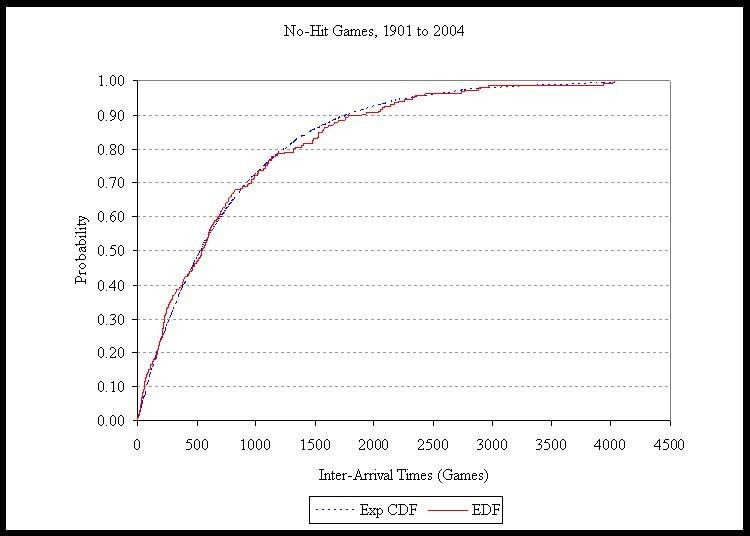
with this algorithm throughout the no-hitter, hitting for the cycle, and triple play data.Bobby Veach (Detroit Tigers, AL) and George Burns (New York Giants, NL) both hit for the cycle on the same day, September 17th, 1920, but in different games; we counted the two events as one game apart. The next no-hitter occurred on May 6th, when Koob’s teammate Bob Groom also pitched a no-hitter against those same White Sox by a score of 3 – 0. It was the 135th game of the season. The inter-arrival time between these two no- hitters was three games. On June 23rd, 1917, Babe Ruth and Ernie Shore of the Boston Red Sox combined to pitch the next no-hitter (Ruth only faced one batter before being ejected for arguing balls and strikes) against the Washington Senators, by a score of 4 – 0. This was the 444th game of the 1917 season, so the inter-arrival time between Groom’s no-hitter and the Ruth/Shore combined no-hitter was 309 games. We calculated the inter-arrival times between successive no-hitters for every season from 1901 through 2004. Using box scores found online at www.retrosheet.org, we verified that each game took place on the date given, then went to the previous day, counted all the wins and losses for all teams, and divided by two. The average inter-arrival time for a no-hitter is 772 games. Similarly, the average inter-arrival times for a cycle and triple play are 720 and 316 games, respectively. At this point we discuss goodness-of-fit tests for the exponentiality of the data. In Figure 4, we present a comparison of the empirical distribution function (EDF) with the fitted exponential cumulative distribution function (CDF) for no-hit games, using the estimated lambda. Similar EDF versus fitted CDF graphs for cycles and triple plays may, of course, be produced.
Figure 4

                  Figure 4: EDF vs. Exponential CDF for No-Hit Games.

Graphically, no-hitter inter-arrival times seem to be well modeled by an exponential. We
now look at formal statistical tests of an exponential model. We first consider Pearson’s
chi-square statistic. It is easy to understand, but as we will indicate, it is problematic for
testing exponentiality. To illustrate the use of the chi-square statistic, we consider the no-
hitter data. A cell count of those inter-arrival times, as well as what we would expect to
see for each cell, is shown in Table 3 below. Each line in the Table shows the interval for
inter-arrival times in which 20 events occurred. For example, 20 no-hitters occurred with
inter-arrival times (x) of 0 x < 56. Similar tables could be constructed for cycles and
triple plays.
Table 3. The Construction of the Chi-square Test Statistic for No-Hitters
IAT
Observed (obs) Expected (exp) (obs - exp)2/exp
<
0 56 20 14.4085 2.1699
56 162 20 24.5716 0.8505
162 221 20 12.2843 4.8462
221 328 20 20.0194 0.0000
328 530 20 31.0046 3.9059
530 638 20 13.5348 3.0882
638 820 20 18.9327 0.0602
820 1132 20 23.6778 0.5713
1132 1654 20 23.3695 0.4858
1654 2762 20 18.4333 0.1332
2762 4029 6 4.6461 0.3945
The sum of the last column in Table 3 is about 16.5. The corresponding p-value, on 10
degrees of freedom, is about 0.09 indicating the exponential null hypothesis for no-hitters
cannot be rejected at the 0.05 significance level. The chi-square test is based on binned
data. Selection of the bin size for data sets is sometimes more of an art than a science.
Some choose to select bins of equal width on the horizontal axis. We have chosen to
create equi-probable bin sizes instead, as this bin-size method has been shown to be
unbiased and more accurate for approximating the null hypothesis (D’Agostino and
Stephens, 1986, pg. 69). The basic idea behind the chi-square test is that the observed
number of points in each bin should be similar to the expected counts. For goodness-of-
fit in general, while the chi-square statistic is easy to understand and implement, it is
problematic and suffers low statistical power. It reduces continuous data into discrete
cells; thus, we lose the resolution of each inter-arrival time. It is well established that
such loss of fidelity makes the chi-square statistic lack power. That is, compared to more
powerful tests, this test will accept a false null hypothesis more often.
Consequently, as noted by D’Agosino and Stephens (1986), with continuous data it is
much more appropriate to use EDF-based statistics that measure the squared distancebetween the EDF and the exponential model, thus relying on the actual value of each
observation. We used the Anderson-Darling A2 statistic for testing the fit of exponential
distributions (as outlined on pages 134 – 135 of D’Agostino and Stephens, 1986, a ‘case
2, rate parameter unknown’ test), and calculated adjusted test statistics of 0.81 for no-
hitters (a p-value between 0.200 and 0.250), 1.03 for cycles (a p-value between 0.100 and
0.150), and a test statistic of 2.73 (a p-value less than 0.0025) for triple plays. For triple
plays, there seems to be a significant departure from exponentiality. This will be further
examined in the next section, where we will use the A2 statistic to examine exponentiality
of our three rare events over eras within the 1901-2004 time frame.
4. Adjusting For Different Eras
Should we make an adjustment for the era in which players play? Baseball has, of course,
changed over the last century. The total number of games played in a single season has
changed, for example, whenever the leagues have expanded with more teams. (In the
modern baseball season, there are 2430 games as each of 30 teams play 162 games. Back
in 1917, by way of contrast, there were only 16 teams who played between 154 and 158
games each, for a total of 1247 games.) Changes in the style of play and players also
impact the number of rare events. There have been periods when pitching was dominant
and other periods when hitting was dominant. Most baseball historians agree that there
have been periods of change, and although everyone might not agree on the exact dates of
different periods, those periods (subsets of the data) can be classified by the eras listed in
Table 4 (see References for source). Also listed are the number of rare occurrences for
each era, by type.
Table 4: Historical Eras of Major League Baseball With Occurrences
Era Years No-Hitters Cycles Triple Plays
Dead Ball 1901 to 1919 43 22 107
Lively Ball 1920 to 1941 20 60 136
Integration 1942 to 1960 30 29 81
Expansion 1961 to 1976 56 31 66
Free Agency 1977 to 1993 37 46 81
Long Ball 1994 to 2004 20 37 40
Each rare event was thus divided into these six eras and the count, mean inter-arrival
times (denoted as Mean IA below), and lambda values were estimated. This information
is shown in Table 5.Table 5: Mean Inter-Arrival Times and Lambda Values Per Era
No- No- Triple Triple
Cycles Cycles
Hitter Hitter Play Play
Mean Mean
Era Seasons Mean IA
IA IA
Dead Ball 19 536 2.26 959 1.16 213 5.63
Lively Ball 22 1344 0.91 449 2.73 199 6.18
Integration 19 788 1.58 798 1.53 285 4.26
Expansion 16 514 3.50 899 1.94 415 4.13
Free
17 889 2.18 747 2.71 444 4.76
Agency
Long Ball 11 1164 1.82 665 3.36 613 3.64
There are clear differences between the eras. For example, during the Dead Ball Era, the
mean inter-arrival time of no-hitters was low, while the mean inter-arrival time of cycles
per year was high. These two trends were reversed during the Lively Ball Era. The mean
inter-arrival time of triple plays did not change significantly during these two eras. The
Expansion Era saw an increase in no-hitters per year, while the recent (and current) Long
Ball Era has seen a drop in the mean inter-arrival time of cycles. Triple play mean inter-
arrival times are up in recent eras.
The Anderson-Darling Goodness-of-Fit Test was applied to each era for each rare event,
to examine whether or not each subset was indicative of exponential behavior (see Table
6). Note that there are significant departures from “exponentiality” in certain subsets of
the data. (We use a significance level of = 0.05 in what follows.) The data for no-
hitters for example, may be exponential in the totality of the data, but is apparently non-
exponential in the ‘Lively Ball’ and ‘Free Agent’ eras. Interestingly in the case of triple
plays, the process is non-exponential as a total process; however, all but one of the eras
fails to reject exponentiality, albeit with different arrival rates. This appears to be
evidence of a non-homogeneous Poisson process. Using a Potthoff-Whittinghill test for
homogeneity of a Poisson process with parameter lambda unknown (Potthoff and
Whittinghill 1966), we reject homogeneity with a very small p-value (Table 6: Anderson-Darling Goodness-of-Fit Tests Stat Era Years A2 n adj A2 adjusted p-value Exponential? all triple plays 1901 - 2004 2.73 511 2.73 < 0.0025 Reject Dead Ball 1901 - 1919 0.48 107 0.48 > 0.25 Do Not Reject Lively Ball 1920 - 1941 0.67 136 0.68 > 0.25 Do Not Reject Integration 1942 - 1960 0.35 81 0.35 > 0.25 Do Not Reject Expansion 1961 - 1976 1.05 66 1.06 = 0.01 Reject Free Agent 1977 - 1993 0.51 81 0.51 > 0.25 Do Not Reject Long Ball 1993 - 2004 0.72 40 0.72 > 0.25 Do Not Reject all Cycles 1901 - 2004 1.03 225 1.03 0.10 < p < 0.15 Do Not Reject Dead Ball 1901 - 1919 2.96 22 3.04 < 0.0025 Reject Lively Ball 1920 - 1941 0.94 60 0.95 0.10 < p < 0.15 Do Not Reject Integration 1942 - 1960 0.72 29 0.73 > 0.25 Do Not Reject Expansion 1961 - 1976 0.72 31 0.73 > 0.25 Do Not Reject Free Agent 1977 - 1993 1.01 46 1.02 0.10 < p < 0.15 Do Not Reject Long Ball 1993 - 2004 0.90 37 0.91 0.15 < p < 0.20 Do Not Reject all No-Hitters 1901 - 2004 0.81 206 0.81 0.20 < p < 0.25 Do not Reject Dead Ball 1901 - 1919 0.96 43 0.97 0.10 < p < 0.15 Do Not Reject Lively Ball 1920 - 1941 1.43 20 1.47 0.025 < p < 0.05 Reject Integration 1942 - 1960 0.95 30 0.97 0.10 < p < 0.15 Do Not Reject Expansion 1961 - 1976 0.63 56 0.64 > 0.25 Do Not Reject Free Agent 1977 - 1993 1.92 37 1.95 0.01 < p < 0.025 Reject Long Ball 1993 - 2004 1.08 20 1.11 0.05 < p < 0.10 Do Not Reject
5. Conclusion
Historical data on no-hitters, cycles, and triples may be used by students to practice their
skill on modeling by the Poisson and/or the exponential distributions. As a part of this
modeling process it is important, of course, that students assess the quality of fit. In this
paper we demonstrated how to study rare baseball events as Poisson processes,
constructing models from the discrete data sets. Using goodness of fit analyses on the
inter-arrival times allowed us to assess the exponentiality of the data.

6. Getting the Data
The no-hitter data is contained in the Excel file nohitters.xls, the cycles data is contained
in the Excel file cycles.xls, and the triple play data is contained in the Excel file triple
plays.xls. The file rarebaseballevents.txt contains a description of the data and, in
particular, a listing of the different variables.

Acknowledgments
The authors wish to thank Travis Smith for assisting with the calculation of triple play
inter-arrival times, Chuck Rosciam and Frank Hamilton for the initial data set for triple
play occurrences, Michael Phillips and Scott Billie for comments on the first draft of this
paper, and Rodney Sturdivant for goodness of fit information and clarification. Finally,
the authors wish to especially thank the referees and editor for their insights and
recommendations.

References
D’Agostino, R. B. and Stephens, M. A. (1986), Goodness-of-Fit Techniques, New York,
NY: Marcel Dekker, Inc.

Devore, J. L. (1995), Probability and Statistics for Engineering and the Sciences, Fourth
Edition, New York, NY: Duxbury Press.

Siwoff, S. (2004), The Book of Baseball Records, 2004 Edition, New York, NY:
Seymour Siwoff, Elias Sports Bureau, Inc.

Potthoff, R. F. and Whittinghill, M. (1966), “Testing for Homogeneity: II. The Poisson
Distribution”, Biometrika, 53(1/2), pp. 183-190.
Internet Sites
Internet site for raw data: www.retrosheet.org (access the ‘Outstanding Feats’ link)
accessed 1 Oct 2004.

Internet site for triple play data: tripleplays.sabr.org/tp_sum.htm accessed 1 Jul 2006.

Internet site for hitting for the cycle facts: www.Baseball-Almanac.com/feats/feats16d.
shtml accessed 1 Oct 2004.

Internet site for no-hit game definition:
mlb.mlb.com/NASApp/mlb/mlb/official_info/official_rules/foreword.jsp accessed 11 Feb
06.

Internet site for baseball eras: www.netshrine.com/era.html accessed 10 Feb 2006.

Michael Huber
Department of Mathematical Sciences
Muhlenberg College
Allentown, PA 18014
U.S.A.
huber@muhlenberg.edu

Andrew Glen
Department of Mathematical Sciences
United States Military Academy
West Point, NY 10996
U.S.A.
andrew.glen@usma.edu

    Volume 15 (2007) | Archive | Index | Data Archive | Information Service | Editorial Board |
   Guidelines for Authors | Guidelines for Data Contributors | Home Page | Contact JSE | ASA
                                           Publications
You can also read