Grid-interactive efficient buildings: Assessing the potential for energy flexibility alongside energy efficiency
←
→
Page content transcription
If your browser does not render page correctly, please read the page content below
Grid-interactive efficient buildings: Assessing
the potential for energy flexibility alongside
energy efficiency
Jared Langevin1, Handi Putra1, Elaina Present2, Andrew Speake2, Chioke Harris2,
Rajendra Adhikari2, and Eric Wilson2

1Lawrence Berkeley National Laboratory
2 National Renewable Energy Laboratory
Motivating question
How much can grid-interactive
efficient building technologies
benefit U.S. electric grid operations?
What is the available electric load “resource” from buildings?

• Buildings comprise 75%
  of U.S. electricity
  demand.
• Demand-side flexibility
  can support variable
  renewable electricity
  penetration cost-
  effectively.
• The magnitude of the
  potential grid resource
  from flexible building
  technologies has not         Comparison of the costs per MWh of shifting renewable energy from
  yet been quantified.         generation sources, and battery storage/distributed energy resources.
                            Aggregated demand-side flexibility resources are found to be cost-effective
                             and frequently cheaper than the generation alternative. Source: McKinsey.
                                                                                                          3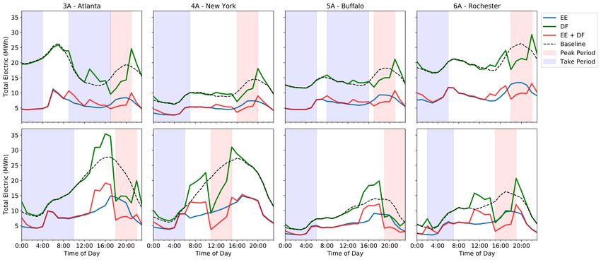
45% Renewable
                                             Electricity Supply
  A guide
  A guidetofor  interpreting
             interpreting (↓62%our
                                2005 results
                          our resultsCO by 2050)                2

             Geographical                    Aggressive
                                             Electricity use Building         Time horizon: Annual and
             granularity: by 22 EIA          Efficiency
                                             segmentation:and  by building    sub-annual results from 2015-
             Electricity Market Module       type (res./com.), end use,       2050; measure relative
             (EMM) regions (no AK/HI).
                                             Electrification
                                             technology                       impacts persist over time.
U.S. Mid-Century Strategy                    (↓10-16% 2005 CO2 by 2050)
(↓80% 2005 CO2 by 2050)

                               Measure grid service:  Measure application:                    Measure adoption:
   2030

          2035

                 2040

                        2045

                                2050

  Measure types:                            Largest Reductions     From
  Energy efficiency            Reduce system annual   All hours/days with                     Full overnight
  (EE); demand                 electricity use and net peak   operational schedules that      adoption, + realistic
     Year (DF);
  flexibility                  period/hour use, increase      shift between summer and        baseline market
    Year
  packaged efficiency          net take period/hour use;      winter based on grid needs;     turnover, + achievable
  and flexibility                                        Building
                               net load shapes assume high          Envelope
                                                              operation at the edge of        sales penetration.
  (EE+DF).                     renewable penetration.         comfort bounds.
                                                                                                                  3
                                                                                                                  4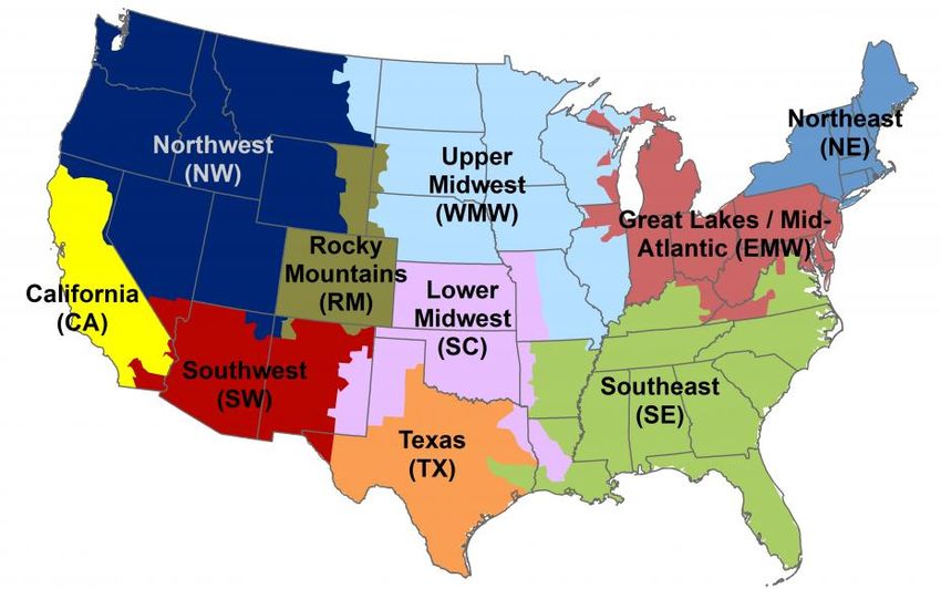
Approach
A bottoms-up stock-and-flow model
of U.S. buildings, combined with
hourly electric loads and simulated
electricity use impacts of efficient and
flexible technologies.
                                           5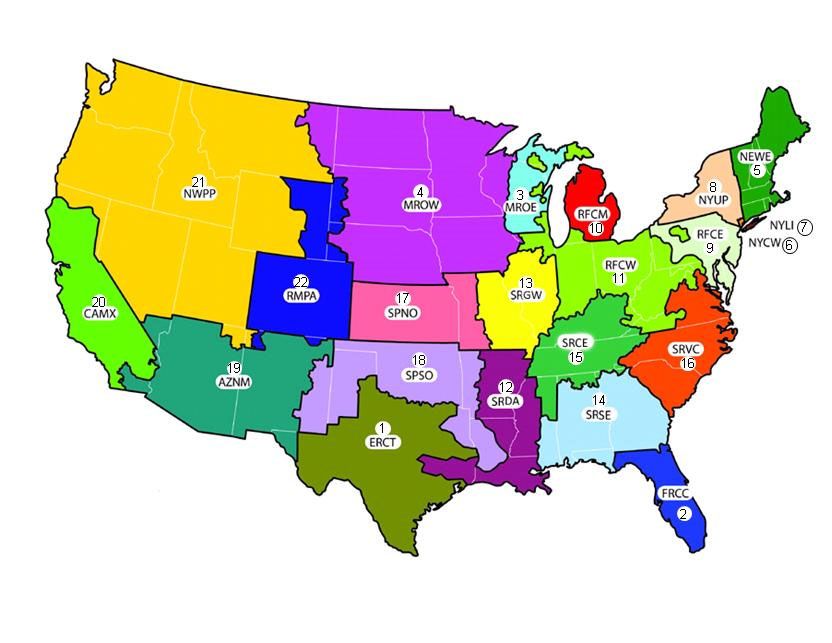
Approach to time-sensitive regional valuation of electricity use

  1. Define measures in technology portfolios
        Energy efficiency (EE), demand flexibility* (DF), and combined EE+DF technology portfolios

  2. Develop 8760 hourly fractions of baseline load by climate zone,
  building type, and end use

  3. Identify seasonal peak period and low demand period by
  electricity market sub-region to inform flexible* measure operation

  4. Simulate measures using ResStock (residential) and OpenStudio
  (commercial) and extract hourly savings fractions from the results

  5. Translate measure impacts to Scout and use Scout to assess regional
  and national portfolio impacts, annually and sub-annually (2015–2050)

* “Flexibility” measures can reduce load during peak hours (“shed”) or move electricity use out of the peak period (“shift”).
  Further details on demand flexibility can be found in the Building Technologies Office Grid-interactive Efficient Buildings Overview.   6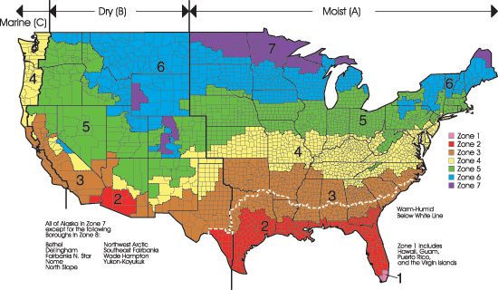
Residential measures were modeled using ResStock

ResStock, a framework for simulating a statistically representative sample of residential buildings in OpenStudio
and EnergyPlus, was used to explore the effect of various measures on hourly residential building energy use.

  Scenario                 Measure Name                   End Use(s)                                 Description
                   Scout “Best Available” ECM                                Current best available residential efficiency ECMs, definitions
                                                        All major end uses
    Energy         portfolio                                                 posted on Scout GitHub repository
Efficiency (EE)    Programmable thermostat (PCT)                             Apply thermostat setups and setbacks while maintaining
                                                             HVAC
                   setups and setbacks                                       temperature setpoint diversity
                   PCT + pre-cooling and heating             HVAC            Decrease/increase temperature set points during peak period
                                                                             Increase temperature setpoint at beginning of take period,
                   Grid-responsive water heater          Water Heating
                                                                             decrease setpoint at beginning of peak period
   Demand
Flexibility (DF)   Grid-responsive washer/dryer,                             Shift washer/dryer cycles and pool pump power to off-peak
                                                           Appliances
                   variable-speed pool pump                                  hours
                                                                             Shift or switch off/unplug some low-priority electronics
                   Low priority plug load adjustments      Electronics
                                                                             during peak hours (e.g., TVs, set top boxes, laptops/PCs)
                   PCT + pre-cool/heat + efficient                           Combine EE HVAC and envelope upgrades with DF HVAC
                                                         HVAC, Lighting
                   envelope and HVAC equipment                               controls
   EE + DF         Grid-responsive cycling/control +    Appliances, WH,      Combine DF WH, appliance, and electronics strategies with
                   efficient equipment                    Electronics        most efficient equipment
                   All remaining EE ECMs                  Refrigeration      Account for efficiency outside of other EE+DF measures

                                                                                                                                               7
Commercial measures were modeled with prototype buildings

The Commercial Prototype Reference Models were used with OpenStudio and EnergyPlus to explore the effect
of various measures on hourly commercial building energy use.

  Scenario               Measure Name                End Use(s)                                  Description
    Energy         Scout “Best Available” ECM        All major end    Current best available commercial ECMs, definitions posted on
Efficiency (EE)    portfolio                              uses        Scout GitHub repository
                   Global temperature adjustment
                                                                      Increase zone temperature set points for one or more peak hours
                   (GTA)
                   GTA + pre-cooling                     HVAC         Decrease zone set points prior to peak period
   Demand          GTA + pre-cooling + storage                        Charge ice storage overnight and discharge during peak period
Flexibility (DF)
                                                                      Dim lighting, and shut off lighting in unoccupied spaces, for one or
                   Continuous dimming                   Lighting
                                                                      more peak hours
                                                                      Switch off low-priority devices (e.g., unused PCs, equipment) for
                   Low priority device switching      Electronics
                                                                      one or more peak hours
                   GTA + pre-cool/heat + efficient                    Combine DF HVAC/lighting strategies with more efficient
                   envelope and HVAC equip.;         HVAC, Lighting   envelope/equipment, daylighting, and controls to maximize EE and
                   daylighting controls + dimming                     DF
   EE + DF         Device switching + efficient                       Combine DF electronics strategy with the most efficient electronic
                                                      Electronics
                   electronics                                        equipment
                                                     Refrigeration,
                   All remaining EE ECMs                              Account for efficiency outside of combined EE+DF measures above
                                                          WH
                                                                                                                                             8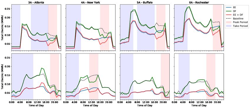
Building-level measure operation addresses system-level needs

• Building-level measure
  operation is modeled in a
  representative city for 14
  ASHRAE/IECC climate zones
  (excludes 1 and 8)
• Representative building types
  capture variations in loads
  and operational patterns
   • Residential: single family
   • Commercial: Large office,
     large hotel, medium office,
     retail, warehouse
• Measures adhere to               ASHRAE/IECC climate zones
  acceptable service thresholds
                                                                9
Fract
Avg. Pk. Hr./Range
Net load shapes vary by region, inform measure operation 0.2 ● Avg. Tk. Hr./Range
Peak Day
Typical Weekday
Summer Month
Winter Month
0 Typical Weekend Intermediate Month
1 3 5 7 9 11 13 15 17 19 21 23
• Regional net system Hour Ending (Local Standard Time)
Period of net peak (high) demand
load shapes for the
year 2050 are used as Hourly
NetNet Load,
Hourly 2050
Load — California
CAMX 2050 Hourly Net Load,
Net Hourly Load2050 — Texas
ERCOT 2050
a reference for
1 1
measure development ●
Avg. Pk. Hr./Range
Avg. Tk. Hr./Range ●
Avg. Pk. Hr./Range
Avg. Tk. Hr./Range
(year with the highest 0.8 0.8
renewable penetration
Fraction Peak Net Load
Fraction Peak Net Load
levels). 0.6 0.6
●
• Flexibility measures 0.4 ● 0.4 ●
●
are designed to ●
remove load during 0.2
●
0.2
Peak Day Summer Month
net peak periods and Peak Day
Typical Weekday
Summer Month
Winter Month Typical Weekday Winter Month
build load during low 0 Typical Weekend Intermediate Month 0 Typical Weekend Intermediate Month
net demand periods 1 3 5 7 9 11 13 15 17 19 21 23 1 3 5 7 9 11 13 15 17 19 21 23
(if possible), flattening Hour Ending (Local Standard Time) Hour Ending (Local Standard Time)
the net load shape.
Net Hourly Load NWPP 2050 Net Hourly Load FRCC 2050
Period of low net demand
1 1 Avg. Pk. Hr./Range
● Avg. Tk. Hr./Range
Data: EIA EMM, projection year 2050 10
0.8 0.8Simulation results yield hourly savings shapes for each measure
• Flexibility measure operation is
defined based on measure Savings Shape
Baseline
configuration and EMM region w/Measure Applied
• Hourly savings fractions are the
difference between the
Electric Load
magnitude of baseline electric
load and electric load with the
measure applied
• Impacts on net peak and low
demand period loads can be
calculated as an average or Net
Low Net Peak
maximum across all relevant Demand Period Period
hours and days within the given 0 4 8 12 16 20
season Time of Day
11Measure results by EMM regions, aggregated to AVERT regions
• Measure building-level operation is assessed relative to system-level load shapes
December 2018
for the 22 EIA Electricity Market Module (EMM) regions
• EMM region results map to the 10 EPA AVERT regions for easier interpretation
Figure 3. Market model supply regions
U.S. EIA EMM regions U.S. EPA AVERT regions
1 ‐ Texas Reliability Entity (ERCT) 12Current limitations
• Primary focus is on technical potential results
• Results do not generally consider market conditions, consumer preferences,
payback period, or price elasticity
• Measures are based on the highest performance technologies currently
available
• Does not include prospective technologies currently in development
• Measure operation is not based on real-time signals
• Flexible operation is defined based on preset net peak (high demand) and
low demand periods set by EMM region
13Context
In 2020, buildings comprise
75% of annual U.S. electricity
demand.
Data: EIA AEO 14Baseline electricity use in 2020 varies widely by region of the U.S.
Annual Electricity Use
800
U.S. Buildings: 2491 TWh
600
Annual Electricity Use (TWh)
400
200
0
Southeast
Mid−Atlantic
Texas
Northeast
California
Upper Midwest
Northwest
Lower Midwest
Southwest
Rocky Mountains
Data: EIA EMM, AEO; Scout 15Daily Avg. Peak Period Demand (GW), Net Peak
0
20
40
60
80
100
120
140
160
Data: EIA EMM, AEO; Scout
Southeast
Mid−Atlantic
Texas
Northeast
Upper Midwest
California
Northwest
Lower Midwest
Peak Summer Demand
Southwest
Rocky Mountains
U.S. Buildings: 458 GW
Daily Avg. Peak Period Demand (GW), Net Peak
0
20
40
60
80
100
120
140
160
Southeast
Mid−Atlantic
Northeast
Texas
Upper Midwest
California
Northwest
Peak Winter Demand
Lower Midwest
Southwest
Peak loads in each region scale with regional total load
Rocky Mountains
U.S. Buildings: 394 GW
16Finding 1
In 2020, buildings could reduce peak
demand by
177 GW (24%*) in the summer and
128 GW (22%*) in the winter.
* Percent of U.S. total peak demand in the indicated season
Data: EIA EMM, Scout 17Peak reduction potential relative to peak demand varies by region
*DRAFT*
Peak Summer Demand Peak Winter Demand
160 160
36% U.S. Buildings: 458 GW U.S. Buildings: 394 GW
Daily Avg. Peak Period Demand (GW), Net Peak
Daily Avg. Peak Period Demand (GW), Net Peak
140 140
35%
120 120
48%
100 100
31%
80 80 Load reduced during
peak demand period
60 60
38%
40 41% 35% 40 28% 35% 29%
32% 35% 35%
36% 33%
32% 33%
20 20 27%
35% 28%
0 0
Southeast
Mid−Atlantic
Texas
Northeast
Upper Midwest
California
Northwest
Lower Midwest
Southwest
Rocky Mountains
Southeast
Mid−Atlantic
Northeast
Texas
Upper Midwest
California
Northwest
Lower Midwest
Southwest
Rocky Mountains
Data: EIA EMM, Scout 18Finding 2
In 2020, buildings could move
15 GW (2%*) of summer and
14 GW (2%*) of winter peak demand
to the hours when electricity demand
is low.
* Percent of U.S. total peak demand in the indicated season
Data: EIA EMM, Scout 19For the technologies considered, load building potential is limited
*DRAFT*
Peak Summer Demand Peak Winter Demand
160 160
U.S. Buildings: 458 GW U.S. Buildings: 394 GW
Daily Avg. Peak Period Demand (GW), Net Peak
Daily Avg. Peak Period Demand (GW), Net Peak
140 140
120 120
100 100
80 80
Load added during low
net demand periods
60 60
40 40
20 20
4% 3% 2% 6%
3% 3% 2% 3% 2% 3% 2% 2% 2% 6% 2% 2% 2% 4% 1% 1%
0 0
Southeast
Mid−Atlantic
Texas
Northeast
Upper Midwest
California
Northwest
Lower Midwest
Southwest
Rocky Mountains
Southeast
Mid−Atlantic
Northeast
Texas
Upper Midwest
California
Northwest
Lower Midwest
Southwest
Rocky Mountains
Data: EIA EMM, Scout 20Finding 3
Efficiency and flexibility are
complementary for peak demand
reduction.
21Efficiency and flexibility are complementary
*DRAFT*
Annual Impacts (2020) Net Peak Period Impacts (2020) Low Net Demand Period Impacts (2020)
200 100 100
Change in Annual Consumption (TWh)
Avg. Change in Hourly Demand (GW)
Avg. Change in Hourly Demand (GW)
Tech. Potential (TP) Increased demand TP−Summer Increased demand TP−Summer
TP−Winter TP−Winter
0 50 50
−3 15 14
0 0
−200
−50 −50
−52
−400
−72 −79
−100 −92 −100 −87
−95
−97
−600 −128
−116
−150 −150
−722
−800 −742
−200 −177
−200
Decreased electricity use Decreased demand Decreased demand
−1000 −250 −250
EE+DF DF EE EE+DF DF EE EE+DF DF EE
Scenario Scenario Scenario
The annual impact of the EE+DF differs from the combined impact of EE
and DF because EE reduces peak electricity demand, and thus reduces the
potential effect of DF measures on peak and total electricity use
Data: Scout
Acronyms: Energy Efficiency (EE), Demand Flexibility (DF) 22Finding 4
Cooling and heating in residential
buildings yield the largest total
electricity use and peak demand
reductions. Commercial plug loads
also offer large reduction potential.
23Residential buildings drive changes in load across metrics
*DRAFT*
Annual Impacts (2020) Net Peak Period Impacts (2020) Low Net Demand Period Impacts (2020)
200 100 100
Change in Annual Consumption (TWh)
Avg. Change in Hourly Demand (GW)
Avg. Change in Hourly Demand (GW)
Tech. Potential (TP) TP−Summer TP−Summer
TP−Winter TP−Winter
0 50 50
−3 15 14
0 0
−200
−50 −50
−52
−400
−72 −79
−100 −92 −100 −87
−95
−97
−600 −128
−116
−150 −150
−722
−800 −742
−200 −177
−200
−1000 −250 −250
EE+DF DF EE EE+DF DF EE EE+DF DF EE
Scenario Scenario Scenario
Residential (New)
54% of average summer peak
Residential (Existing) period reduction and 83% of
Commercial (New) average winter low demand
Commercial (Existing)
period increase comes from
Data: Scout residential buildings
Acronyms: Energy Efficiency (EE), Demand Flexibility (DF) 24Cooling drives peak reduction, water heating adds load
*DRAFT*
Annual Impacts (2020) Net Peak Period Impacts (2020) Low Net Demand Period Impacts (2020)
200 100 100
Change in Annual Consumption (TWh)
Avg. Change in Hourly Demand (GW)
Avg. Change in Hourly Demand (GW)
Tech. Potential (TP) TP−Summer TP−Summer
TP−Winter TP−Winter
0 50 50
−3 15 14
0 0
−200
−50 −50
−52
−400
−72 −79
−100 −92 −100 −87
−95
−97
−600 −128
−116
−150 −150
−722
−800 −742
−200 −177
−200
−1000 −250 −250
EE+DF DF EE EE+DF DF EE EE+DF DF EE
Scenario Scenario Scenario
Heating Water Heating
52% of average summer peak
Cooling Refrigeration period reduction comes from
Ventilation Plug Loads cooling; 56% of average low
Lighting Other
demand period increase comes
Data: Scout from water heating
Acronyms: Energy Efficiency (EE), Demand Flexibility (DF) 25Finding 5
93% of long-run measure impact
potential is captured by 2030 with
replacement at end of life, or
59% with achievable sales
penetration considered.
26Three adoption scenarios considered
Technical Potential Max Adoption Potential Adjusted Adoption Potential
An increasing share of units are
All units are replaced overnight All units are replaced at end of life
replaced at end of life with the
with the efficient/flexible with the efficient/flexible
efficient/flexible alternative, rising
alternative alternative
to 85% of sales by 2035
total stock stock at end of life stock at end of life
each year each year
Stock unit Replaced stock unit
27Technical potential impacts across measure scenarios
*DRAFT*
Annual Impacts (2020) Net Peak Period Impacts (2020) Low Net Demand Period Impacts (2020)
200 100 100
Change in Annual Consumption (TWh)
Avg. Change in Hourly Demand (GW)
Avg. Change in Hourly Demand (GW)
Tech. Potential (TP) TP−Summer TP−Summer
TP−Winter TP−Winter
0 50 50
−3 15 14
0 0
−200
−50 −50
−52
−400
−72 −79
−100 −92 −100 −87
−95
−97
−600 −128
−116
−150 −150
−722
−800 −742
−200 −177
−200
−1000 −250 −250
EE+DF DF EE EE+DF DF EE EE+DF DF EE
Scenario Scenario Scenario
Data: Scout
Acronyms: Energy Efficiency (EE), Demand Flexibility (DF) 28Accounting for adoption reduces potential impacts in 2020
*DRAFT*
Annual Impacts (2020) Net Peak Period Impacts (2020) Low Net Demand Period Impacts (2020)
200 100 100
Change in Annual Consumption (TWh)
Avg. Change in Hourly Demand (GW)
Avg. Change in Hourly Demand (GW)
Tech. Potential (TP) TP−Summer TP−Summer
TP−Winter TP−Winter
0 50 50
−3 15 14
0 0
−200
−50 −50
−52
−400
−72 −79
−100 −92 −100 −87
−95
−97
−600 −128
−116
−150 −150
−722
−800 −742
−200 −177
−200
−1000 −250 −250
EE+DF DF EE EE+DF DF EE EE+DF DF EE
Scenario Scenario Scenario
Max adoption (100% sales/y)
Adjusted adoption (85% sales, 20y)
Data: Scout
Acronyms: Energy Efficiency (EE), Demand Flexibility (DF) 29In the max adoption scenario, most potential is captured by 2030
*DRAFT*
Annual Impacts (2030) Net Peak Period Impacts (2030) Low Net Demand Period Impacts (2030)
200 100 100
Change in Annual Consumption (TWh)
Avg. Change in Hourly Demand (GW)
Avg. Change in Hourly Demand (GW)
Tech. Potential (TP) TP−Summer TP−Summer
TP−Winter TP−Winter
0 50 50
−3 14 14
0 0
−200
−50 −50
−51
−400
−75 −78
−100 −89 −100 −90 −93
−101
−600 −124 −119
−150 −150
−723
−800 −744
−200 −182 −200
−1000 −250 −250
EE+DF DF EE EE+DF DF EE EE+DF DF EE
Scenario Scenario Scenario
Max adoption (100% sales/y)
Adjusted adoption (85% sales, 20y)
Data: Scout
Acronyms: Energy Efficiency (EE), Demand Flexibility (DF) 30By 2050, most impacts are captured in the adjusted adoption scenario
*DRAFT*
Annual Impacts (2050) Net Peak Period Impacts (2050) Low Net Demand Period Impacts (2050)
200 100 100
Change in Annual Consumption (TWh)
Avg. Change in Hourly Demand (GW)
Avg. Change in Hourly Demand (GW)
Tech. Potential (TP) TP−Summer TP−Summer
TP−Winter TP−Winter
0 50 50
−2 15 14
0 0
−200
−50 −50
−51
−400
−100 −100 −79
−90 −88 −95
−104
−600 −125
−116
−150 −136 −150
−800 −782 −200 −200
−806
−209
−1000 −250 −250
EE+DF DF EE EE+DF DF EE EE+DF DF EE
Scenario Scenario Scenario
Max adoption (100% sales/y)
Adjusted adoption (85% sales, 20y)
Data: Scout
Acronyms: Energy Efficiency (EE), Demand Flexibility (DF) 31Conclusion
32An initial step in quantifying the building-grid resource
A quantitative framework was established for time-sensitive, region-specific valuation of building
efficiency and flexibility measures across the U.S.
• Adapts the Scout impact analysis software to enable sub-annual assessment of U.S. building electricity use under
baseline conditions and given efficiency/flexibility measure adoption
• Leverages ResStock (residential) and DOE Prototype Models (commercial) to develop hourly baseline and measure
electric load shapes across 14 climate zones
Initial results show a large potential peak reduction resource from buildings, interactions between
efficiency and flexibility, and regional differences
• In 2020, up to 177 GW U.S. net peak hour load (24% peak) could be removed by efficiency and flexibility measures,
with 722 TWh annual electricity savings (19% total)
• Opportunities to increase load off-peak via flexibility measures (up to 15 GW increase) are reduced by the addition of
efficiency measures (up to 79 GW decrease)
• The EE+DF scenario yields the largest potential peak period reduction, with a substantial reduction in total annual
electricity use—177 GW and 722 TWh, respectively, compared to 97 GW and 3 TWh (DF) or 116 GW and 742 TWh (EE)
Residential and commercial cooling, residential heating, and commercial plug loads show large
potential for impacts on electricity demand
• Cooling yields more than half of maximum peak reduction potential (EE+DF)
• Plug load efficiency and controls (EE, EE+DF) yield the second largest peak reductions and comparable total annual
electricity use reductions to cooling
33Thank you
Jared Langevin jared.langevin@lbl.gov
Chioke Harris chioke.harris@nrel.gov
Scout: scout.energy.gov
ResStock: www.nrel.gov/buildings/resstock.html
Commercial Prototypes:
https://www.energycodes.gov/development/commercial/prototype_models
This work was authored by Alliance for Sustainable Energy, LLC, the manager and operator of the National Renewable Energy
Laboratory for the U.S. Department of Energy (DOE) under Contract No. DE-AC36-08GO28308 and by The Regents of the University
of California, the manager and operator of the Lawrence Berkeley National Laboratory for the DOE under Contract No. DE-AC02-
05CH11231. Funding was provided by the DOE Office of Energy Efficiency and Renewable Energy Building Technologies Office.
The views expressed in this presentation and by the presenter do not necessarily represent the views of the DOE or the U.S. Government.Additional methodology details
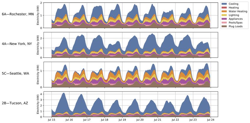
35Example baseline residential load shapes (summer) Rochester, MN New York, NY Seattle, WA Tucson, AZ Data: ResStock 36
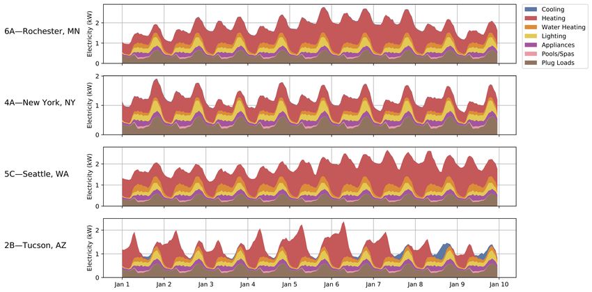
Example baseline residential load shapes (winter)

   Rochester, MN

   New York, NY

   Seattle, WA

   Tucson, AZ

Data: ResStock                                        37
Example baseline commercial loads (summer, medium office)
                                                                          End Use Load Profiles for a August week
                                                                            Building type: MediumOfficeDetailed
                           Tampa,    FL
                           2A−Tampa, FL
                                                                                                                                               Lighting
                     150
                                                                                                                                               Plug Loads
 Electricity [kWh]

                                                                                                                                               Heating
                     100                                                                                                                       Cooling
                                                                                                                                               Ventilation
                      50

                       0
                                Aug−21         Aug−22   Aug−23   Aug−24               Aug−25          Aug−26        Aug−27   Aug−28   Aug−29

                           New
                           4A−NewYork,
                                  York, NYNY
                     160
 Electricity [kWh]

                     120

                      80

                      40

                       0
                                Aug−21         Aug−22   Aug−23   Aug−24               Aug−25          Aug−26        Aug−27   Aug−28   Aug−29

                           Seattle,    WA
                           4C−Seattle, WA
 Electricity [kWh]

                     100

                      50

                       0
                                Aug−21         Aug−22   Aug−23   Aug−24               Aug−25          Aug−26        Aug−27   Aug−28   Aug−29

                           Rochester,     MN
                           6A−Rochester, MN
                     150
 Electricity [kWh]

                     100

                      50

                       0
                                Aug−21         Aug−22   Aug−23   Aug−24               Aug−25          Aug−26        Aug−27   Aug−28   Aug−29

Data: EnergyPlus/OpenStudio Commercial Prototype simulations                                                                                                 38
Example commercial baseline loads (winter, medium office)
End Use Load Profiles for a January week
Building type: MediumOfficeDetailed
Tampa,
2A−Tampa,FL
Tampa, FL
FL
Lighting
Plug Loads
Electricity [kWh]
100 Heating
Cooling
Ventilation
50
0
Jan−23 Jan−24 Jan−25 Jan−26 Jan−27 Jan−28 Jan−29 Jan−30 Jan−31
New
New York,
4A−NewYork, NY
NY
York, NY
150
Electricity [kWh]
100
50
0
Jan−23 Jan−24 Jan−25 Jan−26 Jan−27 Jan−28 Jan−29 Jan−30 Jan−31
Seattle,
4C−Seattle,WA
Seattle, WA
WA
150
Electricity [kWh]
100
50
0
Jan−23 Jan−24 Jan−25 Jan−26 Jan−27 Jan−28 Jan−29 Jan−30 Jan−31
Rochester,
Rochester, MN
MN
6A−Rochester, MN
300
Electricity [kWh]
200
100
0
Jan−23 Jan−24 Jan−25 Jan−26 Jan−27 Jan−28 Jan−29 Jan−30 Jan−31
Data: EnergyPlus/OpenStudio Commercial Prototype simulations 39Residential measure scenario load impacts
*DRAFT*
Atlanta New York Buffalo Rochester, MN
Total Electric Load (MWh)
January 24
Total Electric Load (MWh)
August 24
Time of Day Time of Day Time of Day Time of Day
Data: ResStock, GEB Measures 40Residential EE and DF measures: key assumptions
EE Measure Approach DF Measure Approach
Central AC Upgrade to SEER 18 AC from any lower SEER. Pre-heat to 140°F during take period (second
Water heater take period, if applicable), then return to 125°F
Upgrade to SEER 22/HSPF 10 from any lower ASHP, setpoint.
ASHP or (in some cases) electric furnaces.
Pre-cool/pre-heat by 3°F starting 4 hours
Applied 10 hour daytime set-back of 8°F in winter and before the peak, then set-back/set-up of 4°F
set-up of 7°F in summer, and 8 hour nighttime set- Thermostat relative to original setpoint during peak period.
Thermostat controls back of 8°F in winter and 4°F in summer. Thermostat DR setpoints take precedence over
Daytime set-back only weekdays for 43% of homes. EE thermostat setpoints.
Refrigerator Upgrade to EF 22.2. Baseline schedules are generated as normal
Clothes washer, (randomly based on distributions). Then event
Walls Upgrade to R-13 cavity with R-20 external XPS. clusters during peak are shifted after peak if
Clothes dryer, possible, if not then before peak if possible, if
Roofs Upgrade unfinished attic insulation to R-49. Dishwasher not then left as-is.
No change in total energy use.
Air sealing Upgrade to 1 ACH50 with mechanical ventilation.
All energy use during peak period is removed
Upgrade to: U-0.17, 0.49 SHGC in AIA CZ1; U-0.17,
and added uniformly to energy use during the
Windows 0.42 SHGC in AIA CZ2; U-0.17, 0.27 SHGC in AIA CZ3; Pool pump (first) take period.
U-0.17, 0.25 SHGC in AIA CZ4–5.
No change in total energy use.
Floors Upgrade wall and ceiling insulation. Of peak period electronics energy usage:
• 11% is shifted to the 2 hour period following
HPWH Upgrade to high EF, 80-gal HPWH.
the peak, representing discharging batteries
during peak.
Clothes washer Upgrade to IMEF 2.92, usage level maintained. Electronics • 4% is removed, representing zero standby
Clothes dryer Upgrade to CEF 3.65, usage level maintained. power consumption (i.e., advanced power
strip controls).
Dishwasher Upgrade to 199 rated annual kWh, usage maintained. Total energy use decreases.
Pool pump Upgrade to (0.75 hp) 1688 rated annual kWh.
Electronics Decrease total annual energy use by 50%. 41Commercial measure scenario load impacts (medium office)
*DRAFT*
Atlanta New York Buffalo Rochester, MN
Total Electric Load (MWh)
January 24
Total Electric Load (MWh)
August 24
Time of Day Time of Day Time of Day Time of Day
Data: EnergyPlus/OpenStudio Commercial Prototypes, GEB Measures 42Commercial EE and DF measures: key assumptions
EE Measure Approach DF Measure Approach
Medium and Large Offices upgrade to follow AEDG Reduce lighting loads by 30% for occupied
50% guidelines for floor, roof, and exterior walls for Lighting spaces and 60% for unoccupied spaces
medium offices. Large Hotel uses the AEDG 50% for during the peak hours.
Envelope highway lodging. Warehouse uses the AEDG 30%
Reduce plug loads by 20% for occupied
for small warehouses. Retail Stand-Alone uses the
AEDG 50% for medium and big-box retail. Plug loads spaces and 100% for unoccupied spaces
during the peak hours.
Upgrade to follow AEDG guidelines on lighting using
Increase global temperature by 5°F in the
Lighting the same building type mapping as the envelope Global temperature summer and decrease by 2°F in the winter.
upgrade. adjustment The adjustment occurs during peak hours.
Upgrade to follow AEDG guidelines on equipment
Pre-cool by 2°F four hours before the peak
Plug loads power density according to the same building type
period. Passive pre-cooling applies to the
mapping as the envelope upgrade. Pre-cooling Medium Office, Stand-Alone Retail, and
Upgrade to higher COP HVAC equipment. Large Warehouse prototypes.
Hotel already has an efficient air-cooled chiller.
Implement a 6.7 COP charging chiller and
Large Office chiller is upgraded to 7 COP. All other
HVAC building types (e.g., medium office, retail, and
ice storage on the HVAC plant loop. Charge
ice storage 12AM to 6AM. Discharge ice
warehouse) have their 2-speed DX cooling unit Ice storage storage during the peak period. The active
upgraded to 4 COP and its burner efficiency to 0.99.
ice storage option applies to the Large Hotel
Upgrade to match “high” commercial refrigeration and Large Office prototypes.
performance in “EIA Updated Buildings Sector
Refrigeration Appliance and Equipment Costs and Efficiency
Appendix C,” 2018.
Upgrade to match “high” commercial heat pump
water heater performance in “EIA Updated Buildings
Water heating Sector Appliance and Equipment Costs and
Efficiency,” 2018.
43Integration of data inputs and outputs in Scout Translating between
Demand Flexibility in Scout technologies and
sectors
Input data
CDIV Base load, TSV
ASH CZ.
Intermediate ->EMM price, and metric
->EMM
data mapping emissions settings
mapping
shapes
Output data
TXT JSON TXT CMD
CDIV = Census Division
EMM = EIA Electricity Baseline Baseline Baseline
Market Module Region annual annual
ASH CZ = ASHRAE energy energy
8760s
(by EMM)
△M
90.1 climate zones (by CDIV) (by EMM)
ECM = Energy Measure
JSON Python Python JSON
Conservation Measure load
savings
shape • Change in energy,
carbon, cost
Scout Efficient JSON Efficient • Annually, per
ECM annual 8760s season
attributes energy (by EMM)
(by EMM) • Full day, peak, take
• Single, multiple hrs.
JSON Python Python
• Sum, max., avg.
44Additional results
45Individual measure impacts during the summer
*DRAFT*
Decrease in Annual Consumption (TWh)
Decrease in Annual Consumption (TWh)
● EE+DF ● EE ● DF ● EE+DF ● EE ● DF
150 ● ● 150 ● ●
● ●
4 3 2
100 ● 100 ●
● ● ● ●
● ●
2
50 ●●
●
● 50 ●● ●
●
● ● ●
● ● ●
● ● ● ● ●
● ● ● ●●●
●
● ● ● ●●
●
●
●● ● ●●
●
0 ●●
● ●
●●
●
●
●
●
● 5 0 ●●●●
●
● ●
●●
●● ●●● ● ●● ● ●
1 543 1
−50 −50
0 10 20 30 −20 −15 −10 −5 0 5 10
Avg. Decrease in Summer Net Peak Demand (GW) Avg. Increase in Summer Net Take Demand (GW)
1 Preconditioning (DF−R) 1 Water Heater (DF−R)
2 ASHP (EE−R) 2 HPWH (EE+DF−R)
3 Plug Loads (EE+DF−C) 3 Ice Storage (DF−C)
4 Plug Loads (EE−C) 4 HVAC+Ice (EE+DF−C)
5 HVAC+GTA+Precool (EE+DF−C) 5 Pool Pump (DF−R)
TWh)
TWh)
● EE+DF ● EE ● DF ● EE+DF ● EE ● DF
461 Preconditioning (DF−R) 1 Water Heater (DF−R)
2 ASHP (EE−R) 2 HPWH (EE+DF−R)
Individual measure impacts during the winter 3
4
Plug Loads (EE+DF−C)
Plug Loads (EE−C)
3
4
Ice Storage (DF−C)
HVAC+Ice (EE+DF−C)
5 HVAC+GTA+Precool (EE+DF−C) 5 Pool Pump (DF−R)
*DRAFT*
Decrease in Annual Consumption (TWh)
Decrease in Annual Consumption (TWh)
● EE+DF ● EE ● DF ● EE+DF ● EE ● DF
150 ● ●
150 ● ●
● ●
32
100 ● 100 ●
● ●
●
● 4 ●
●
1
50 ●
●
● ●●
50 ●
●● ●
● ●
● ●●● ● ●● ●
● ●
● ● ● ● ● ●●
● ●
● ● ●●
●●● ● ● ●
●
●
●●
●●●●● ● ●
● ●●
●
0 ●
●
●● ● ●● ● 0 ●●●
● ● ● ●
5 543 2 1
−50 −50
0 5 10 15 20 −15 −10 −5 0 5
Avg. Decrease in Winter Net Peak Demand (GW) Avg. Increase in Winter Net Take Demand (GW)
1 HPWH (EE+DF−R) 1 Water Heater (DF−R)
2 ASHP (EE−R) 2 Preconditioning (DF−R)
3 Plug Loads (EE+DF−C) 3 Ice Storage (DF−C)
4 HPWH (EE−R) 4 HVAC+Ice (EE+DF−C)
5 Preconditioning (DF−R) 5 Clothes Dryer (DF−R)
47Annual Electricity Use (TWh)
0
200
400
600
800
Southeast
Mid−Atlantic
Texas
Annual
Northeast
Data: EIA EMM, AEO; Scout
California
Upper Midwest
Northwest
Annual Electricity
Lower Midwest
Southwest
ElectricityUse
Use
Rocky Mountains
U.S. Buildings: 2491 TWh
Daily Avg. Peak Period Demand (GW), Net Peak
0
20
40
60
80
100
120
140
Southeast
Mid−Atlantic
Peak
Texas
Northeast
Upper Midwest
California
Peak Summer
Northwest
Lower Midwest
Southwest
Summer Demand
Demand
Rocky Mountains
U.S. Buildings: 458 GW
Daily Avg. Peak Period Demand (GW), Net Peak
0
20
40
60
80
100
120
140
Southeast
Mid−Atlantic
Northeast
Peak
Texas
Upper Midwest
Peak Winter
California
Northwest
Lower Midwest
Winter Demand
Southwest
Demand
Rocky Mountains
U.S. Buildings: 394 GW
Baseline electricity use in 2020 varies widely by region of the U.S.
48Annual Electricity Use (TWh)
0
200
400
600
800
Southeast
Mid−Atlantic
Texas
Annual
Northeast
Data: EIA EMM, AEO; Scout
California
Upper Midwest
Northwest
Annual Electricity
Lower Midwest
Southwest
ElectricityUse
Use
Rocky Mountains
Daily Avg. Peak Period Demand (GW), Net Peak
0
20
40
60
80
100
120
140
Southeast
Mid−Atlantic
Peak
Texas
Northeast
Upper Midwest
California
Peak Summer
Northwest
Lower Midwest
Southwest
Summer Demand
Demand
Rocky Mountains
Daily Avg. Peak Period Demand (GW), Net Peak
0
20
40
60
80
100
120
140
Southeast
Mid−Atlantic
Northeast
Peak
Texas
Upper Midwest
Peak Winter
California
Northwest
Other
Lower Midwest
Cooling
Heating
Lighting
Winter Demand
Southwest
Ventilation
Plug Loads
Demand
Refrigeration
Rocky Mountains
Water Heating
Electricity use differences between regions are driven by end uses
49Annual Electricity Use (TWh)
0
200
400
600
800
Southeast
Mid−Atlantic
Texas
Annual
Northeast
Data: EIA EMM, AEO; Scout
California
Upper Midwest
Northwest
Annual Electricity
Lower Midwest
Southwest
ElectricityUse
Use
Rocky Mountains
Daily Avg. Peak Period Demand (GW), Net Peak
0
20
40
60
80
100
120
140
Southeast
Mid−Atlantic
Peak
Texas
Northeast
Upper Midwest
California
Peak Summer
Northwest
Lower Midwest
Southwest
Summer Demand
Demand
Rocky Mountains
Daily Avg. Peak Period Demand (GW), Net Peak
0
20
40
60
80
100
120
140
Southeast
Mid−Atlantic
Northeast
Peak
Texas
Upper Midwest
Peak Winter
California
Northwest
Lower Midwest
Winter Demand
Southwest
Demand
Residential
Rocky Mountains
Commercial
The share of electricity use by building sector also varies by region
50The buildings sector drives U.S. annual and peak electric loads Data: EIA EMM/AEO, Scout 51
The buildings sector drives U.S. annual and peak electric loads

                                                                  52
The buildings sector drives U.S. annual and peak electric loads
53The buildings sector drives U.S. annual and peak electric loads
54The buildings sector drives U.S. annual and peak electric loads
55Efficiency and flexibility are complementary and conflicting
*DRAFT*
Annual Impacts (2020) Net Peak Period Impacts (2020) Low Net Demand Period Impacts (2020)
200
Change in Annual Electricity Use (TWh)
Avg. Change in Hourly Demand (GW)
Avg. Change in Hourly Demand (GW)
Technical Potential (TP) 100 TP−Summer 100 TP−Summer
0 TP−Winter TP−Winter
50 50 15 14
−3
−200 0 0
−50 −50
−400 −52
−100 −100 −72 −79
−97 −92 −87 −95
−600 −116
−150 −128 −150
−722 −200 −177 −200
−800 −742
−250 −250
−1000
−300 −300
−1200 −350 −350
EE+DF DF EE EE+DF DF EE EE+DF DF EE
Scenario Scenario Scenario
-722 TWh: 19% of total -177 GW: 24% of total -72 GW: Efficiency
U.S. electricity use in summer U.S. non- reduces opportunity to
2020 coincident peak in 2020 build load
Data: Scout
Acronyms: Energy Efficiency (EE), Demand Flexibility (DF) 56You can also read