Measurement and Simulation of Energy Use in an Office Building with Hybrid Ventilation
←
→
Page content transcription
If your browser does not render page correctly, please read the page content below
Measurement and Simulation of Energy Use in an Office Building
                  with Hybrid Ventilation
Hans Martin Mathisen, Dr.Ing.
SINTEF Energy Research;
Hans.M.Mathisen@sintef.no, www.sintef.no

Rasmus Høseggen, Ph.D.-student,
NTNU, Department of Energy and Process Engineering;
Rasmus.Hoseggen@stud.ntnu.no, www.ept.ntnu.no/ek/

Sten Olaf Hanssen, Professor,
NTNU, Department of Energy and Process Engineering;
Sten.O.Hanssen@ntnu.no, www.ept.ntnu.no/ek/

KEYWORDS: Hybrid ventilation, simulations, measurements, energy use, control strategies.

SUMMARY:
The objective of this work is to demonstrate the consequences on energy use by adjusting control parameters in
a building with hybrid ventilation and displacement air supply. The interest for hybrid ventilation has increased
during the last years. Hybrid ventilation has mostly been used in schools, but near Trondheim in Norway an
office building with displacement ventilation was erected during 2002. The building has a culvert embedded in
the ground and under the building, and displacement ventilation in the office rooms. For more than a year the
building’s energy use for heating, ventilation and electric equipment has been monitored. In addition,
measurements of room temperatures and the presence of people were carried out. These latter parameters are
important in order to calibrate a simulation model. The energy use seemed to differ from what was expected in
the design phase. To study why the calculated energy use differed from the measured values, simulations were
carried out with an integrated simulation model using ESP-r. The results show that the allowed temperature
swing in the room has significant influence on the energy use. The simulations indicate that it is possible to save
up to 25 % of the total energy use for heating by adjusting the allowance in temperature swing. In comparison,
improving the heat exchanger efficiency by 10 %, the energy savings were 7-11 %. The improved energy
performance did not significantly affect the thermal comfort.

1. Background and objectives
The interest in hybrid ventilation has increased during the last years (Schild, 2003), but has so far mostly been
used in schools. However, near Trondheim in Norway an office building with hybrid ventilation was erected
during 2002. This provided an opportunity to measure energy use in a building with this type of ventilation and
to compare simulations with real data. The simulation model can further be used to study how adjusting of
control parameters and changing the system design, can influence on energy use and thermal indoor environment
in a hybrid ventilated building.
The objective of the work presented in this paper is to demonstrate the consequences on energy use by adjusting
control parameters in a building with hybrid ventilation and displacement air supply.

2. Method
Hourly measurements were carried out during one year from summer 2003 to summer 2004 and included water
based energy for space heating and ventilation together with electricity for lighting and equipment. Simulation of
measured values was done by modelling the complete building. Validation of the simulations was done by
comparing with measurements. The last step was to use the simulation model to evaluate the effect of different
changes related to room temperature control, heat recovery and type of ventilation.
3. Description of the building and technical installations
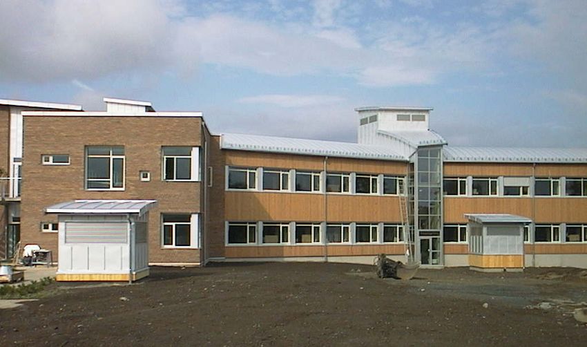
The case building presented in this paper belongs to Nord-Trøndelag College (HiNT) in Levanger, located 80 km
north of Trondheim, Norway. The building was ready for occupation in August 2002. It has a common wing
with meeting rooms and educational areas. Two other wings are office areas, see Figure 1. To simplify the
project, only one of the office wings (the HiNT wing) was used in the study. The building has two storeys, see
Figure 2. It has no basement, but a culvert for supply of ventilation air is embedded in the ground along the
central axis of the wing. A more detailed description of the building, measurements and LCC calculations can be
found in (Mathisen, 2004).
N
HiNT wing
HiNT wing
Figure 1. Plan view of the building showing the Figure 2. The east façade with the air intake towers
common area and the two office wings. “31” is in the foreground. The right tower supplies the office
the air intake tower wing. The glazed area is the stairwell. The tower
above the stairwell is the exhaust air tower.
The HiNT-wing has a net area of 478 m2, of which 269.5 m2 are used as office cells. Each cell is about 9 m2. The
gross area of the wing is 835 m2, of which 112 m2 is used for culvert, air intake tower and exhaust tower.
The hybrid ventilation is of so called culvert type. In principle it is constructed as shown in Figure 3. The ducts
from the culvert to the rooms are buried in the ground beneath the floor. At the façade the ducts turn 90o
upwards. The ducts end in a damper placed inside the supply air terminal device. The air terminals are placed at
the floor beneath the windows. Air to the first floor is supplied through enclosed ducts at the inside of the façade.
Supply air terminal device for displacement Embedded
ventilation. Damper for controlling airflow culvert
Air intake tower
rate One terminal for each office/module
First floor
Ground
floor
Filter, fan, heat recovery and heating coil
Damper for bypassing coils
Figure 3. Culvert in principle and a section through the building. 1: Air intake tower. 2: Air intake culvert.
3: Air distribution culvert. 4: Stairway. 5: Corridors. 6: Exhaust air tower.
From the offices the air flows through grilles placed close to the ceiling and into the corridor. Exhaust of air
takes place through corridors and stairway up to the tower on the roof. The exhaust air tower contains a heat
recovery coil and a fan.
Radiators are placed beneath each window. None of the offices have mechanical cooling. Each office cell has a
presence detector and a temperature sensor and a digital controller unit that controls heating, ventilation and
lighting. Venetian blinds are automatically and simultaneously controlled for each façade, with a possibility for
individual control. Bus is used for communication.Figure 4 shows the ventilation and controller system in principle. The supply and exhaust fans are controlled by
the pressure difference between the culvert and the corridor at the ground floor, i.e. the fans should keep the
pressure difference constant. When there is no heating demand for the ventilation air and the outdoor
temperature exceeds 15 °C, the bypass dampers opens to reduce the pressure drop.
Exhaust
air tower
Exhaust air Presence and
fan temperature detectors
T
Office
Damper room
(bypass)
Digital room
controller
Cirkulation Controller Radiator
pump for supply air Office Office
room room
temperature
Air intake tower
Dampers for
airflow rate
100%
T T T
T
q +
Flow
+ T
Supply Damper
air fan T (bypass)
Filter Differential
pressure SP=21 21.3 22.3
Controller for transducer
pressure in culvert Heating Cooling
Figure 4. Ventilation system in principle and the control strategy for the room controller.
The dampers in the supply air terminal devices control the air flow rate to each room. They operate as follows:
Normally they close at 4 pm. At 6 am open to give approximately 25 m3/h (2.8 m3/hm2) of air . When a person
enters the room they open to give 43 m3/h (4.8 m3/hm2). If the room air temperature exceeds the set-point they
open further. When the temperature is one degree above the set-point they are fully opened and give about 200
m3/h (22 m3/hm2).
If the room air temperature is above the set-point, the dampers also open at night. Total airflow rate supplied to
the HiNT-wing is 8 600 m3/h. 800 m3/h is drawn from toilets without any heat recovery.
4. Description of the simulation model
The simulation model is implemented in the building/plant simulation program ESP-r (ESRU, 2000). The model
is a whole-building model. Figure 5 shows how the model appears in the cad-window in the ESP-r Project
Manager.
Figure 5. The whole-building simulation modelConstruction elements
The modelling of the building elements are done by investigating the construction drawings. In principle, the
building envelope is very well insulated, far better than required by the national building code. However, the
extensive occurrences of thermal bridges make the U-value increase significantly. Table 1 shows the basic
U-values and the thermal bridge corrected U-values calculated by methods described by the Norwegian
guidelines and EN-ISO-6946 (EN-ISO 6946, 1996).
Table 1. U-values for selected building constructions
Building Basic U-value Thermal bridge corrected
construction [W/m2K] U-value [W/m2K]
External walls 0.18 0.33
Roof 0.12 0.17
Floor on ground 0.15 0.17
Windows 1.31 1.40
The air intake culvert and the air distribution culvert are embedded ground coupled concrete ducts. The floors
and the walls are modelled as a concrete layer and an insulation layer. One meter of earth is also included in
these constructions. The construction is coupled to a constant temperature in the ground; 10 °C underneath the
building and 5 °C outside the building. This is a fairly rough simplification, but gives a good approximation to
the complex physics in the ducts (Wachenfeldt, 2003). This approximation is also done for the floor
constructions with ground coupling.
Air flow network model
Supply air is taken through the culvert before it is mixed with extract air from the zone in the heat recovery unit.
The mixing of the two air flows is a simple approach to model the heat exchanger, and is not meant to be a
recirculation of air. If necessary, the air is preheated to the given set-point. The air flows further into the air
distribution culvert, which can also be seen in Figure 5 under the office building. From the distribution culvert
the zones are supplied with air by fans. The model has a total of eight fans supplying the eight air-conditioned
zones. From the offices the air flows through an opening to the corridor and from the corridor into the stairway,
where the air is extracted by two fans. One fan feeds the heat recovery zone, and the other leads the rest to the
outside. By replacing stack and wind effects with fans, the model supposes that the hybrid ventilation system
works ideally at all times with regard to airflow rates and temperature control.
The model has a free cooling system. When the outside dry bulb temperature exceeds 15 °C, the air is by-passed
the heat recovery unit. In Figure 6 that means that damper 4 opens, while dampers 2 and 3 are shut. Damper 1
opens to fulfil the mass balance.
(1 − η ) ⋅ qm Symbols :
Stairway = fan
Hallway
= damper
Qint
qm = air mass flow
η = heat exchanger efficiency
η ⋅ qm Qint= internal gains
= radiator heating
Qrad
Offices
Heat re-
Air covery Inf = 0.2ach
intake Qint
Ambient culvert Pre-
air node heating
Qrad
qm
Air
distribution
culvert
Figure 6. Principal scheme of the simulation model with an air flow networkAir supply control
The air flow is controlled both by the presence of people and temperature in the specific zones. The minimum air
flow for an occupied zone is approximately 4.8 m3/ hm2 and 2.8 m3/hm2 in an empty zone during the working
hours. If the temperature raises above the set-point the air volume increases proportionally with the temperature
until full opening at 22 m3/hm2. The presence of people is fixed in the control strategy, and is given by the
occupational load in the internal gains. Table 2 outlines the air control strategy.
Table 2. Air flow rates at different times of a working day. Set-points (SP) change over the year and room-type.
See Figure 7 for the SP-values. The office rooms are occupied 8-10 and 13-16.
Min airflow Max airflow [m3/hm2]
Time Control range [oC ]
[m3/hm2] (Temp. controlled)
0-6 0.0 22.0 SP + 1.5 °C → SP + 2.0 °C
6-8 2.8 22.0 SP + 0.3 °C → SP + 1.3 °C
8-10 4.8 22.0 SP + 0.3 °C → SP + 1.3 °C
10-13 2.8 22.0 SP + 0.3 °C → SP + 1.3 °C
13-16 4.8 22.0 SP + 0.3 °C → SP + 1.3 °C
16-24 0.0 22.0 SP + 1.5 °C → SP + 2.0 °C
Other days 0.0 22.0 SP + 1.5 °C → SP + 2.0 °C
Set-points for heating and ventilation
The set-points for heating and ventilation vary over the year. The office cells have individual set-points for
heating, while the set-points for the common area and the supply air are set by the operator. All rooms have 2 K
night set-back relative to the set-point during working hours. Figure 7 shows the actual monitored set-points that
were used in the simulations. The reason for the increased set-point for the supply air during winter period is due
to complaints about draught against ankles.
Internal gains
The internal gains are persons (occupational load), equipment and lighting. In every zone type, except for one
server room, all internal loads are shut down during night hours and weekends. Figure 8 shows the internal gains
during a working day.
24 40
office cells offices
hallway / common area 35 hall/common
23 supply air
Heat gain [W/m2]
30
Set-point [oC]
22
25
21 20
15
20
10
19
5
18 0
Jan Feb Mar Apr May Jun Jul Aug Sep Oct Nov Dec 2 4 6 8 10 12 14 16 18 20 22 24
Figure 7. Set-points for the office cells, the Figure 8. The internal gains in the office cells
hallways/common areas and the supply air. and the hallway/common area
Climate
Ideally, the climate data should have been recorded at the location in the same period the energy consumption
measurements were done. As this data were insufficient, it was decided to use the hourly Test Reference Year
(TRY) data produced by the program Meteonorm (Meteonorm, 2004) for Trondheim Airport Vaernes, located
30 km south of Levanger. The official air temperature measurements from the meteorological station at Vaernes
(MET.no, 2005) show that the annual average temperature during the time of this study was 1,5 °C above the
standard year. The TRY values however, are somewhere between the standard year and the actual
measurements. Table 3 shows the monthly average air temperatures from Vaernes (met.no), the TRY and the
standard year, respectively.Table 3. Monthly average air temperatures [°C] for the time of study, TRY and the standard year
jan feb mar apr may jun jul aug sep oct nov dec avg
met.no -3.4 -0.4 2.7 7.9 9.2 13.1 17.6 14.2 10.7 3.8 2.5 0.5 6.5
TRY -4.4 -4.3 -0.1 4.4 10.8 15.1 16.5 15.3 10.6 6.4 0.7 -3.0 5.7
Standard -3.4 -2.5 -0.1 3.6 9.1 12.5 13.7 13.3 9.5 5.2 0.5 -1.7 5.0
Simulation strategy
The simulations were run month by month to compare directly to measured values. The heat recovery unit had a
failure during December and January. This has been taken into account in the calibrated simulation model by
reducing the efficiency to 20 %.
5. Simulations
Basic model
The results for monthly heating of the rooms and the ventilation air from the calibrated basic simulation model
are given in Figure 9. Table 4 shows the total energy use and the relative agreement to measured values.
18000
room heating
16000 ventilation
14000
Energy use [kWh]
12000
10000
8000
6000
4000
2000
0
Jan Feb Mar Apr May Jun Jul Aug Sep Oct Nov Dec
Month
Figure 9. Energy use distributed on room heating and ventilation air preheating for each month. First bar is
measured values and the second is the results from the simulation model.
Effect of adjusting the control range
The objective of this section is to study the impact of allowing the room temperature to glide somewhat more
than in the basic model before full damper opening occurs in the air supply terminals. The same set-points for
room and ventilation air temperature as in the basic model are used. The only modification from the basic model
is that the heat exchanger efficiency is constant throughout the year. Two cases are simulated with 45 % and
55 % heat exchanger efficiencies, respectively.
90 000 Dead Control
η = 45%
η = 55% band range
85 000
100%
Energy use [kWh]
80 000
0 1 2 3 4
Flow
75 000
70 000
65 000
60 000 20 21 22 23 24 25 26
0 1 2 3 4 Temp. oC
Control range Heating Cooling
Figure 10. Energy use as a function of the control range Figure 11. The different control ranges. The set-
and efficiency of the heat recovery unit. The meaning of point (SP) is 21 °C. The dead band (DB) is 1 °C.
the control ranges are explained in Figure 11.Comparing measured energy use with results from Figure 10 indicates that increasing the dead band up to 1 K
and allowing 3 K temperature glide before full damper opening, makes it possible to save about 25% of the total
energy use for heating.
Excessive temperature
Hours with room air temperature above 26 °C increase about 6 hours during a year when changing the upper set-
value from 23 °C to 24 °C, and additional 10 hours for 25 °C. However, temperatures above 26 °C occur less
than 50 hours during a year within working hours, but will exceed 50 hours with higher upper set-values.
Other simulations
Table 4 summarizes some of the simulations carried out in this study. The first two rows in Table 4 are the
measured values and the simulated values, respectively, as presented in Figure 9. The third row (Basic_CR3) is a
slight modification of the basic model. The only difference from the basic model is that the control range is set to
22-25 °C instead of 21.3-22.3 °C. The fourth row presents the results from a model where the set-points and
technical solutions are in accordance with the designed values, i.e. the supply air is held at 20 °C the entire year
and the heat exchanger efficiency is constantly 45 %. The “Improved design” configuration has a control range
of 22-25 °C and a heat exchanger efficiency at 55 %. The latter two configurations presuppose that the draught
problems are solved.
Table 4. Comparison of different cases
Supply air Ventilation Total Rel. difference
Room heating
Case temperature, air preheating energy from measured,
[kWh]
summer/winter [kWh] use [kWh] total [kWh]
Measured values As Figure 7 26 317 61 874 88 192 -
Basic model As Figure 7 23 071 70 289 93 360 + 6%
Basic_CR3 As Figure 7 23 673 49 108 72 782 - 17 %
Designed 20/20 27 922 43 455 71 377 - 19 %
Improved design 19/20 25 775 32 867 58 642 - 34 %
6. Discussion
The simulated basic model and the measured values agree well. It must be remembered that measured values has
uncertainty due to measurement accuracy and missing data in some periods. The simulations are based on a
climatic year different from the real climate. Further, the real case’s set-points differ from room to room and
frequently during the year, while the values used in the simulation model are monthly averages of monitored
values. The calculated U-values due to taking the thermal bridges into account are another uncertainty in the
simulation model.
May and October are the only months the simulation model determines less energy use than the measurements.
This can be explained by the fact that these months have a higher average outdoor air temperature (see Table 3).
In comparing measurements and simulations, the total energy use for heating agrees better than the separate
energy use for heating the rooms and the ventilation air. This can be explained by the narrow dead band between
radiator heating and cooling by increasing the ventilation air. For instance, if the simulation model over-predicts
room temperature by as little as 0.3 °C (21.3 °C instead of 21.0 °C see Figure 4) this leads to ventilation air
heating demand instead of room heating demand.
The embedded ducts have a heat loss that is difficult to estimate because the temperature in the ground varies
during the year. On the contrary, the lost heat leads to higher temperature in the ground that might reduce the
heat loss through the floor.
The “Designed” and “Improved design” cases require that the ventilation works without draught problems.
Today the supply air temperature is increased by the operator in order to reduce the draught sensation. High
supply air temperature gives increased heat loss from the culvert, the embedded ducts, and reduced ventilation
efficiency (Mundt, 2004). If the room temperature is allowed to glide more before full opening of the dampers,
the airflow rate is reduced. Reduced airflow rate implies lower air velocity in the vicinity to the air terminal. On
the other hand, higher temperature difference between room air and inlet air increases the density differences andhence the acceleration of the air. However, higher room air temperature implies that higher air velocities are
accepted before the users sense draught. (Skistad, 2002), (Mathisen, 1989).
7. Conclusions
• Annual total specific energy use is measured to be 161 kWh/m2 heated gross area, of which
111 kWh/m2 are hydronic space heating and heating of ventilation air.
• The simulations carried out in ESP-r agree well with the measurements.
• The thermal environment is satisfactory during summertime with less than 50 hours with temperature
above 26 °C. Even if the temperature glide is allowed up to 25 °C before full damper opening, the
number of hours with over temperature increases with only a few hours.
• The total airflow rates during working hours are relatively large; this is due to the fact that the control
range for the room temperature was only 1 K. On cold days this means that preheating in addition to
recovered heat is necessary. If the dead band between radiator heating and cooling by increased
ventilation is expanded to 1 K, and the temperature is allowed to glide 3 K before full opening, it is
possible to save about 25 % of the total energy use for heating compared to the measurements.
• Increasing the heat exchanger efficiency from 45 to 55% will save about 7-11% of the total energy use,
depending on the control range. That is, the energy use is more dependent on the control range for the
room temperature than the heat exchanger efficiency.
• The simulations show that if the type of hybrid ventilation system presented in this paper is well
designed and operated, moderate energy use can be obtained.
References
ESRU (1999). “ESP-r: a building and plant energy simulation environment, User Guide Version 9 Series, ESRU
Publication,” University of Strathclyde, Glasgow, United Kingdom
EN ISO 6946 (1996). Building components and building elements Thermal resistance and thermal transmittance
Calculation Method, Oslo, Norway
Mathisen H.M. (2004). “Evaluering av hybrid ventilasjon – Casestudie Nordlåna Røstad – Hovedrapport”
(Evaluation of Hybrid Ventilation – Case study Nordlåna Røstad), SINTEF TR A6024, SINTEF Energy
Research, Trondheim, Norway
MET.no (2005). Norwegian Meteorological Institute, Online Climate Database, http://eklima.met.no
Meteonorm (2004). Global Meteorological Database for Solar Energy and Applied Meteorology,
http://www.meteotest.ch/en/produkte/
Mundt E., Mathisen H.M., Nielsen P.V. and Moser A. (2004). ”Ventilation Effectiveness”, REHVA Guidebook
No 2, Brussels, Belgium
Schild P.S., Dokka T.H., Mysen M. and Tjelflaat P.O. (2003). “Bygningsintegrert ventilasjon – en veileder”
(Building Integrated Ventilation - A Guidline), Økobygg, Oslo, Norway
Skistad H., Mundt E., Nielsen P.V., Hagström K. and Railio J. (2002). ”Displacement ventilation in non-
industrial premises”, REHVA Guidebook No 1, Brussels, Belgium
Wachenfledt B.J. (2003). “Natural Ventilation in Buildings – Detailed Prediction of Energy Performance”, PhD
Thesis, Norwegian University of Science and Technology, Trondheim, Norway
Mathisen H.M. (1989). "Analysis and Evaluation of Displacement Ventilation", PhD Thesis, Norwegian
University of Science and Technology, Trondheim, NorwayYou can also read