Real-time parameter inference in reduced-order flame models with heteroscedastic Bayesian neural network ensembles
←
→
Page content transcription
If your browser does not render page correctly, please read the page content below
Real-time parameter inference in reduced-order flame
                                                 models with heteroscedastic Bayesian neural network
                                                                      ensembles

                                                      Ushnish Sengupta ∗                    Maximilian L. Croci ∗          Matthew P. Juniper
                                                   Department of Engineering              Department of Engineering      Department of Engineering
arXiv:2011.02838v1 [cs.LG] 11 Oct 2020

                                                    University of Cambridge                University of Cambridge        University of Cambridge
                                                        Cambridge, UK                          Cambridge, UK                  Cambridge, UK
                                                      us271@cam.ac.uk                        mlc70@cam.ac.uk               mpj1001@cam.ac.uk

                                                                                                   Abstract

                                                      The estimation of model parameters with uncertainties from observed data is an ubiquitous
                                                      inverse problem in science and engineering. In this paper, we suggest an inexpensive and
                                                      easy to implement parameter estimation technique that uses a heteroscedastic Bayesian
                                                      Neural Network trained using anchored ensembling. The heteroscedastic aleatoric error of
                                                      the network models the irreducible uncertainty due to parameter degeneracies in our inverse
                                                      problem, while the epistemic uncertainty of the Bayesian model captures uncertainties which
                                                      may arise from an input observation’s out-of-distribution nature. We use this tool to perform
                                                      real-time parameter inference in a 6 parameter G-equation model of a ducted, premixed flame
                                                      from observations of acoustically excited flames. We train our networks on a library of 2.1
                                                      million simulated flame videos. Results on the test dataset of simulated flames show that the
                                                      network recovers flame model parameters, with the correlation coefficient between predicted
                                                      and true parameters ranging from 0.97 to 0.99, and well-calibrated uncertainty estimates.
                                                      The trained neural networks are then used to infer model parameters from real videos of
                                                      a premixed Bunsen flame captured using a high-speed camera in our lab. Re-simulation
                                                      using inferred parameters shows excellent agreement between the real and simulated flames.
                                                      Compared to Ensemble Kalman Filter-based tools that have been proposed for this problem
                                                      in the combustion literature, our neural network ensemble achieves better data-efficiency and
                                                      our sub-millisecond inference times represent a savings on computational costs by several
                                                      orders of magnitude. This allows us to calibrate our reduced order flame model in real-time
                                                      and predict the thermoacoustic instability behaviour of the flame more accurately.

                                         1       Introduction

                                         Complex, nonlinear physical models of engineering systems give rise to challenging inverse problems which
                                         require the estimation of unknown model parameters from observations, along with uncertainty quantification.
                                         With the growing popularity of digital twins [1], there is also a need to do bring down the computational
                                         cost of parameter inference such that these models may be updated in real-time using the latest sensor
                                         observations. Traditional filtering-based techniques require the system to be simulated in parallel, which
                                         becomes infeasible if the underlying model is computationally expensive to simulate. Amortized inference
                                         using neural networks [2] circumvents this problem by having an expensive offline training phase, where a
                                         surrogate of the approximate posterior p(θ|z) is learnt from a library of simulator-generated observations zi
                                         corresponding to input parameters θi , typically using normalizing flow-based methods [3] [4]. The surrogate
                                         can then be rapidly evaluated online to perform parameter inference on new observed data.
                                             ∗
                                                 The first two authors contributed equally to this work.

                                         Machine Learning and the Physical Sciences workshop at the 34th Conference on Neural Information Processing Systems
                                         (NeurIPS 2020), Vancouver, Canada.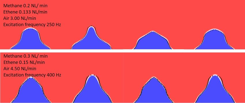
The physical model that motivated this paper is a reduced order kinematic model for flames that captures
the response of a ducted premixed flame to acoustic perturbations, known as the G-equation[5]. An accurate
description of this response is necessary because the interplay between acoustic waves and the heat release rate
of the flame can lead to undesirable thermoacoustic instabilities, which have presented an obstinate challenge
to designers of high-energy density combustors [6]. Previous studies [7][8] have reported that calibrating the
parameters of the G-equation model parameters using the Ensemble Kalman Filter can make it quantitatively
accurate and reproduce the experimentally observed behaviour of acoustically forced flames. To achieve a
converged estimate of the parameters, however, the ensemble Kalman filter needs a long sequence of flame
observations, the assimilation of which requires that multiple instances of the G-equation solver be run for
hours. The Ensemble Kalman Filter can also get trapped in local optima if the ensemble of simulations is
initialized poorly. Our current study evaluates the feasibility of performing the same task accurately with a
drastically lower compute budget and fewer observations, using an amortized neural network-based inference
technique.

2     Data: experiments and simulations
2.1   Experimental observations of ducted premixed Bunsen flame

                                      Figure 1: The experimental setup.

Figure 1 shows a schematic of the experimental setup. It has a premixed, laminar Bunsen flame inside a
cylindrical enclosure, with an optical access window for a high-speed camera. A loudspeaker, driven by
an amplified sinusoidal signal, is mounted upstream of the flame for acoustic forcing. Experiments were
performed at different fuel compositions (methane: ethene ratios), flow rates, excitation frequencies (250 - 450
Hz) and excitation amplitudes. The flame dynamics are recorded with a Phantom v4.2 CMOS camera at a
resolution of 1200x800 pixels and a frame rate fs = 2500 fps. Thresholding is applied to the grayscale frames
to detect a thick band around the flame front. For each row of pixels in the image, the mean x coordinate of the
pixels within the band, weighted by their intensities, is used to compute a single x coordinate. Cubic splines
with 28 knots are then fitted through the (x, y) coordinates to obtain a unique x location of the flame front
corresponding to every y. The vector of flame front x-coordinates could be used directly as input observations
for inference. We are interested in modelling the variation of the instantaneous heat release rate and flame
areas are a better proxy for heat release rates. We therefore divide the domain vertically into 90 horizontal
strips and compute the flame area corresponding to the flame segment it contains. Each frame is thus converted
into a 90-dimensional vector of flame areas. 10 successive frames from a video recording are stacked to form
an observation zi , a 900-long vector from which we need to infer the G-equation parameters θi likely to have
generated it.

2.2   Reduced order G-equation model

The G-equation is a kinematic flame model that models the flame as an infinitely-thin front propagating into
unburnt gases at a fixed speed sL [5]. It uses a level-set formulation where the flame front is defined as the
G = 0 contour of the two-dimensional time-varying G-field G(x, y, t). The G-equation is written as
                                           ∂G
                                              + v.∇G = sL |∇G|                                              (1)
                                           ∂t
Here, flame speed sL = sL,u (1 − Mk κ) is a function of the unstretched flame speed sL,u , the flame curvature
κ and the Markstein length Mk . The prescribed velocity field v = (U (x) + v 0 )j + u0 i is the sum of a
                                                       2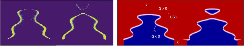
constant parabolic base flow U (x) = U (1 + va − 2va x2 ) and continuity-obeying velocity perturbations
v 0 (x, y, t) = U a sin(St(Ky − t)) and v 0 (x, y, t) = − U aβKSt xcos(St(Ky − t)). U is a characteristic flow
speed, va determines the parabolicity of the base flow velocity profile, a is the amplitude and U/K the
phase speed of velocity perturbations, St is the Strouhal number and β is the aspect ratio of the unforced
flame. Any flame dynamics that can be generated by the G-equation may be uniquely specified by a set of 6
Figure 2: Left: Experimentally observed dynamics of an acoustically excited flame. Right: A flame generated
by the G-equation.
parameters which we need to infer from experimental observations: K, a , Mk , va , St and β. To generate
our simulation dataset, we sample quasi-randomly from the prior over parameters P (θ), assumed uniform
within the hyper-rectangle defined by the following bounds 0 ≤ K ≤ 2.5, 0 ≤ a ≤ 1.0, 0.02 ≤ Mk ≤ 0.08,
0.0 ≤ va ≤ 1.0, 0.5 ≤ St ≤ 125.0, 2.0 ≤ β ≤ 10.0 and 0.08 ≤ fs ≤ 0.20. For each sampled set of
parameters θi , the G-equation is solved using the LSGEN2D solver [9] and the solution is time marched until
a limit cycle is reached. The simulated flames then undergo the same data pre-processing steps outlined above
for the experimental flames. The x-coordinate of the zero level set is identified for each y, the flame area
vectors are computed for each frame and sequences of 10 frames, each separated from adjacent ones by a
phase difference so as to match the experimental frame rate fs , are stacked to form observation vectors zi
corresponding to θi . We compute limit cycle oscillations for 11800 different θi -s, from which we generate 2.4
million simulated observations zi . 10% of the θi -s (240000 zi -s) are held out in the test set.
3 Inference using heteroscedastic Bayesian Neural Networks
We assume that the posterior p(θ|z) can be modelled as a Bayesian neural network µ(z; w) with heteroscedas-
tic Gaussian aleatoric uncertainty σ(z; w). Although the Gaussian assumption may seem restrictive, previous
studies as well as our physical intuition indicate that the posterior here is unimodal and weakly correlated.
Multi-modality, too, can be dealt with in this framework by using a Bayesian mixture density network instead
of a simple neural network, but this has not been considered here. The neural network has a simple MLP
architecture of 3 fully connected ReLU layers with 100 units each and a final sigmoid layer that forces the
output parameters as well as the predicted aleatoric noise to lie between 0 and 1 (input observations and output
parameters are both re-scaled into the range [0, 1]). A He normal [10] prior is used for the neural network
parameters.
The size of the dataset calls for scalable approximate inference techniques for training the neural network.
Here we use approximately Bayesian ensembling using randomized maximum a posteriori (MAP) sampling
[11]. Ensembling had already been shown [12] to be empirically effective at providing calibrated estimates
of uncertainty for neural networks and the randomized MAP sampling approach grounds this in Bayesian
theory. For the j-th neural network ensemble member, we draw a sample from the prior distribution over
neural network parameters (assumed multivariate normal) wanc,j ∼ N (0, Σprior ) and compute the MAP
estimate corresponding to a prior re-centered at wanc,j . Given ND parameter-observation pairs {θi , zi }, we
minimize the following loss function for the j-th neural network
ND ND
−1/2
X X
Lossj = (θi − µj (zi ))T σj (z)−1 (θi − µj (zi )) + log(|σj (z)|) + kΣprior (wj − wanc,j )k22 (2)
i=1 i=1
The prediction of a trained ensemble with M neural networks is therefore a mixture of M Gaussians, each
centered at µj (zi ) with a variance of
Pσj (z). For computational
P convenience,P we approximate this mixture
1 1 1 2 1 2
P
as a single Gaussian with mean M j µj and variance M j σj + M j µj − ( M j µj ) , following
similar treatment in [12]. This also allows us to decompose the total predictive uncertainty into an aleatoric
component (first term) and an epistemic component (second and third terms).
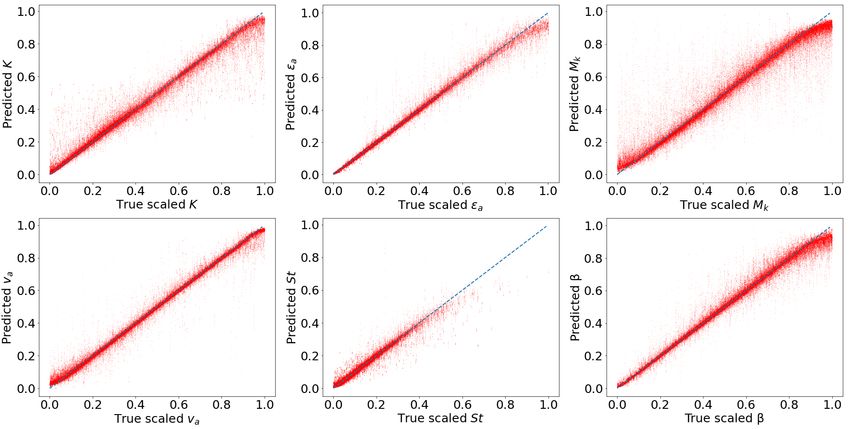
3Figure 3: Scatter plots of true parameters (scaled) versus predicted parameter values for simulated test data.
Figure 4: Experimentally observed flames (black dots) overlaid on re-simulated G-equation flames.
4 Results
Results on the test set of simulated observations (Figure 3) indicate that accurate estimates of G equation
parameters are recovered by the neural network. The correlation coefficient ρ between true and predicted
parameter values are 0.982, 0.994, 0.971, 0.993, 0.976 and 0.990 for K, a , Mk , va , St and β, respectively.
Estimates of parameter uncertainty are also well-calibrated, with particularly high uncertainties in K and St
predicted for datapoints with low a -s (amplitude of perturbation), which is physically sensible, as it is not
possible to recover these parameters from an unperturbed flame. Given a 10-frame observation vector as input,
the neural network takes ~0.1 milliseconds on our Tesla K80 GPU to make parameter predictions. Including
the pre-processing time for thresholding, spline fitting and area calculation, predictions can therefore be made
in less than a millisecond for every few seconds of acquired video data.
We use the trained network to predict parameter values for 10 experimental flame videos and re-simulate the
flames using mean predicted parameter estimates. The re-simulated flames match the dynamics of the real
flames closely (Figure 4). The root mean squared difference between x-coordinates of simulated and real
flame fronts, averaged over all y positions and frames, ranges from 0.0171 to 0.068 units (burner radius is 1
units). The mean re-simulation RMSD across all the flame videos is 0.043 units.
5 Conclusions
We use a heteroscedastic Bayesian neural network ensemble to calibrate the parameters of the G-equation, a
reduced-order model for predicting the dynamics of premixed flames, based on observations. The ensemble
was trained on 2.1 million simulated flame observations and results on the test set of simulated flames show
that parameters are recovered accurately by the network from only 10 frames of flame data. Reasonable
estimates of parameter uncertainties were also obtained. We then use the network to infer parameters from
4high-speed video footage of acoustically excited Bunsen flames in our lab. Re-simulating the flames using
inferred parameters reveals a close agreement between the model output and experimental data, validating
our data assimilation. Compared to the Ensemble Kalman filter used for this task in the literature, our neural
network based technique can perform assimilate flame videos much more rapidly and obtain accurate parameter
estimates using fewer observations.
There are several promising avenues for future work. We will look at assimilating data from more realistic
industrial flame configurations as well as integrating our calibrated reduced-order flame models into higher-
level thermoacoustic network models of an entire combustor.
Broader Impact
This work will lead to better-designed high-energy density combustors, such as those found in rocket and
aircraft engines, by enabling designers to assimilate data from experiments more quickly, refine thermoacoustics
models more accurately, and therefore design out thermoacoustic oscillations more reliably.
Acknowledgments and Disclosure of Funding
This project has received funding from the European Union’s Horizon 2020 research and innovation program
under the Marie Skłodowska- Curie grant agreement number 766264.
References
[1] A. Fuller, Z. Fan, C. Day, and C. Barlow. Digital twin: Enabling technologies, challenges and open
research. IEEE Access, 8:108952–108971, 2020.
[2] Kyle Cranmer, Johann Brehmer, and Gilles Louppe. The frontier of simulation-based inference. Pro-
ceedings of the National Academy of Sciences, 2020. ISSN 0027-8424. doi: 10.1073/pnas.1912789117.
URL https://www.pnas.org/content/early/2020/05/28/1912789117.
[3] Danilo Rezende and Shakir Mohamed. Variational inference with normalizing flows. In International
Conference on Machine Learning, pages 1530–1538, 2015.
[4] Stefan T Radev, Ulf K Mertens, Andreass Voss, Lynton Ardizzone, and Ullrich Köthe. Bayesflow:
Learning complex stochastic models with invertible neural networks. arXiv preprint arXiv:2003.06281,
2020.
[5] Ann P Dowling. Nonlinear self-excited oscillations of a ducted flame. Journal of fluid mechanics, 346:
271–290, 1997.
[6] T Lieuwen. Modeling premixed combustion-acoustic wave interactions: A review. Journal of propulsion
and power, 19(5):765–781, 2003.
[7] Hans Yu, Thomas Jaravel, Matthias Ihme, Matthew P Juniper, and Luca Magri. Data assimilation and
optimal calibration in nonlinear models of flame dynamics. Journal of Engineering for Gas Turbines and
Power, 141(12), 2019.
[8] Hans Yu, Ushnish Sengupta, Matthew Juniper, and Luca Magri. Time-accurate calibration of a thermoa-
coustic model on experimental images of a forced premixed flame. Bulletin of the American Physical
Society, 64, 2019.
[9] Santosh Hemchandra. Dynamics of turbulent premixed flames in acoustic fields. PhD thesis, Georgia
Institute of Technology, 2009.
[10] K. He, X. Zhang, S. Ren, and J. Sun. Delving deep into rectifiers: Surpassing human-level performance
on imagenet classification. In 2015 IEEE International Conference on Computer Vision (ICCV), pages
1026–1034, 2015.
[11] Tim Pearce, Mohamed Zaki, Alexandra Brintrup, Nicolas Anastassacos, and Andy Neely. Uncertainty
in neural networks: Bayesian ensembling. In International Conference on Artificial Intelligence and
Statistics, 2020.
5[12] Balaji Lakshminarayanan, Alexander Pritzel, and Charles Blundell. Simple and scalable predictive
uncertainty estimation using deep ensembles. In Advances in neural information processing systems,
pages 6402–6413, 2017.
6You can also read