A model to calculate electrostatic charge structure of eruptive clouds from volcanic eruptions
←
→
Page content transcription
If your browser does not render page correctly, please read the page content below
E3S Web of Conferences 196, 02001 (2020)                                  https://doi.org/10.1051/e3sconf/202019602001
STRPEP 2020

 A model to calculate electrostatic charge structure of eruptive
 clouds from volcanic eruptions

     Vladimir Uvarov 1 , Rinat Akbashev2 , Pavel Firstov1,2 and Nina Cherneva1 ,
 1
   Institute of Cosmophysical Research and Radio Wave Propagation FEB RAS, Kamchatskiy kray, Paratunka,
 Russia
 2
   Kamchatka Branch of FRC GS RAS, Petropavlovsk-Kamchatksiy, Russia

              Abstract. The paper proposes a model to calculate electrostatic charge structure of
              an eruptive cloud (EC) based on the response of atmospheric electric field (AEF EZ )
              strength during cloud passage near an observation site. The model provides high identity
              of calculated and experimental data for complex configurations of EC electrostatic
              charges. Examples of calculation of EC structures from Shiveluch volcano (Kamchatka)
              eruptions are given. They were estimated with the help of the developed model based on
              the records of AEF EZ response at the distances of 45 and 113 km.

              Key words: volcano, eruption, eruptive cloud, electrostatic charge

 1 Introduction
 Generation of atmospheric electrostatic field (AEF) is associated with multiple processes of planetary
 and local scales. Global electric circuit is determined by global lightning sources [1]. Moreover, at the
 local level, AEF is connected with such local parameters, affecting electrization mechanism, as con-
 ductivity, temperature, viscosity, electron and ion concentration, ionization source strength, aerosol
 concentration and content and others [2]. Cloud electrization of meteorological origin primarily refers
 to local sources of AEF variations [3].
      For the Kamchatka peninsula and a number of other regions of the globe where volcanic activity
 manifests itself, EC electrization is an intensive additional factor. The electrization occurs as the result
 of volcanic eruption [4, 5]. The main difference between the clouds of meteorological origin and ECs
 is that ECs, initiated by volcanic explosive activity, are loaded with significant volume of fine grained
 ash and aerosols and have high temperature contrast at cloud-atmosphere boundary [6, 7]. Moreover,
 depending on the character of explosive activity, volcanic ash content, amount of water dissolved in
 magma and so on, EC electrization is conceivable within wide limits of charge value and with different
 polarization [8–13]. These circumstances as well as the interaction of EC boundary with the clouds of
 meteorological origin cause lightning activity. Lightning stroke location by modern techniques allows
 one to trace EC propagation [14, 15].
    Corresponding author: nina@ikir.ru
 The paper was carried out within the framework on the subject «Dynamics of physical processes in active zones of near space
 and geospheres» (AAAA-A17-117080110043-4) and supported by RFBR Grant 19-05-00543 (AAAA-A19-119041790002-0).

© The Authors, published by EDP Sciences. This is an open access article distributed under the terms of the Creative Commons
Attribution License 4.0 (http://creativecommons.org/licenses/by/4.0/).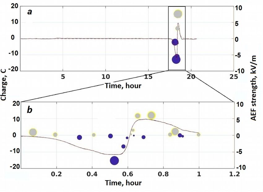
E3S Web of Conferences 196, 02001 (2020)                        https://doi.org/10.1051/e3sconf/202019602001
STRPEP 2020

      EC evolves during its propagation: fractionation during weighted component sedimentation,
 aerosol formation, its temperature decrease [16, 17] that is reflected in EC electrostatic structure
 [12, 13]. Near-field electrostatic processes in EC are indirect signs of eruption character [18] whereas
 in the far-field zone, the conditions of EC propagation under wind effect make significant impact on
 its electrization.
      In the course of investigation of EC electric structure, observations of atmospheric electric field
 vertical component (AEF EZ ) by ground-based electrostatic fluxmeters were very popular [7, 13, 19,
 20]. When interpreting the obtained data and calculating EC charge, one of the following models
 is usually applied: field of one effective charge, field of uniformly charged ellipsoid body [21] or
 dipole field [5]. Such an electric structure of a cumulonimbus cloud is represented by at least 4
 main space charges, two main ones of which form a vertical dipole [22]. Simulation of a field of
 differently originated clouds is quite illustrative and thus is widely used for qualitative description.
 Field simulation by uniformly charged ellipsoid is used, as a rule, for massive cloud formations [23].
 In order to describe such a model, 6 parameters (3 diameters and 3 orientation angles) are required,
 but in most cases it is difficult to calculate them.
      EC formed under wind effect are usually characterized by small vertical dimensions, significant
 extent along the drift direction and small crosswise dimensions. As opposed to the vertical electric
 structure of meteorological clouds, horizontal structure is typical for EC. In this case, to describe field
 sources, we need to apply several ellipsoids of different polarity and orientation that makes the model
 more complicated and hardly suitable for quantitative analysis.
      When describing a symmetric dipole, one needs 7 components: 6 coordinates of charge position
 and one for charge value. However, in the majority of cases, real aero-electric structures are asymmet-
 ric. Thus, it is necessary to add a unipolar charge to the dipole for the approximation to be satisfactory.
 As a result we have that in a simplest case we need to obtain 8 unknown quantities from experimental
 values for quantitative application of such a model. Applying such a model, EC electric structure with
 significant horizontal dimensions should be described by several dipoles. That complicates model
 application and makes it problematic to use it for EC electric structure investigation.

 2 Volcanic globule

 To construct a model of a charged EC, we refer to the known notions in electrostatics. The basis
 of them is detection of a uniformly charged volume element the field of which can be approximated
 by point charge field. Combination of such fields into more complicated configurations (dipoles,
 quadruples etc.) allows one to approximate a field of arbitrary configuration with required accuracy.
 As the simplest element of EC electrostatic structure we take a compact uniformly-charged space of
 diameter Dc and charge Q which is called «volcanic globule» (VG). As a rule, the observed typical
 VG dimensions are significantly less than the distance from a source to the observation site. Thus, we
 approximate VG field by point charge field with sufficient accuracy. For the VG field with significant
 horizontal dimensions we introduce an additional parameter taking into account its extention.
      Such an approach allows us to turn to the model approximating EC electric field by the superpo-
 sition of fields of separate electrostatic structures of simplest forms, VG. Under certain assumptions,
 BG parameters are determined from the data obtained by ground-based electrostatic fluxmeters. Thus,
 description of EC electrostatic structure is reduced to the superposition of VG set charges fields. Vol-
 canic activity is reflected indirectly in EC, thus, EC electrostatic field decomposition on the basis of
 partial fields of separate VG may give an idea on volcanic activity character if we take into account
 the evolution processes occurring as the result of its motion along the transfer direction under wind
 effect.

                                                     2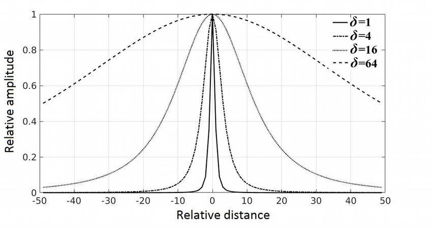
E3S Web of Conferences 196, 02001 (2020) https://doi.org/10.1051/e3sconf/202019602001
STRPEP 2020
3 Description of the model
A mathematical model always contains some limitations since it represents a certain degree of ide-
alization of a real situation. In this case, to construct our model, we have to assume that relaxation
processes are absent. It is fair if the characteristic time of relaxation evolution of EC separate compo-
nents is more than that of their position change.
We consider rectangular coordinates with the origin at the point of sensor location with the ver-
tical axis Z and horizontal axis X, oriented along VG motion, and axis Y perpendicular to it (Fig.1).
Dynamics of VG motion in such a coordinate system is determined by wind velocity ν at the height z
and time t − tniar is the moment of the closest distance to VG, x = ν · (ti − tniar ).
When making such a choice of coordinates, VG trajectory projection on the ground surface is at
the distance y from the axis X. VG center position is determined by the vector R = n · x2 + y2 + z2 ,
where n is a unit vector directed from the origin of coordinates to VG with the coordinates x, y, z.
Extreme value of field intensity module Emax is achieved at the distance Rmin = y2 + z2 .
Figure 1. Volcanic globule motion in the model coordinate system
Air conductivity is many orders less than that of the ground. Thus, when constructing the model,
we assume that ground conductivity is infinite. Then, VG charge field over the Earth surface is de-
scribed by the superposition of fields of two equal charges of opposite signs located at equal distances
over and under the ground surface and being direct reflections of each other. As a result, the field at
the Earth surface level has only a vertical component and can be described by the expression:
Ez = A · Ψ, (1)
In this expression the first factor which is determined by charge value and the minimum distance
to a VG is the field amplitude independent of time and VG location.
Qz
A= , (2)
2πε0 · R3min
where Rmin is the minimum distance from a detector to the horizontal projection of VG trajectory, ε0
is the dielectric constant.
3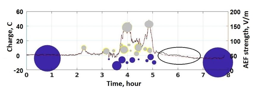
E3S Web of Conferences 196, 02001 (2020)                           https://doi.org/10.1051/e3sconf/202019602001
STRPEP 2020

     The second factor describes the characteristics of VG field with a unit charge moving under wind
 effect at the height z along a straight line parallel to axis X with velocity ν.
                                                                   2 −3/2
                                           Ei         ν(ti − textr )
                                   Ψi =        = 1+                           ,                           (3)
                                          Emax              δ

 where ti , textr is the current time and the time of VG position at the minimum distance from an ob-
 servation site, δ is the extension parameter defining VG effective size and controlling curve Ψi form
 (Fig.2) under the condition that VG motion corresponds to Fig.1.

 Figure 2. Extension function curves for different parameter δ values

     From the obtained ratios (1 – 3) we can make the following conclusions:
 • VG field is described by an even function becoming a unit at the extremum point and going to zero
   at infinity;
 • at the extremum point, field value is equal to A;
 • when the height z is known and the distance from a sensor to the horizontal projection of trajectory
   y is the shortest, applying experimental data we can find VG charge according to (2):

                                                  2πε0 · R3min
                                               Q=A             ,                                (4)
                                                       z
    Charge sign is determined by A position relatively the field average value and the width of the
 curve Ψ, describing field structure, is determined by effective extension parameter δe f f .

 4 VG extension parameter
 As the VG charge from ratio (4) is determined we can determine VG characteristic dimension applying
 expression (3) by searching for an optimal approximation M = AΨ(δopt ) of Ez data sampling that is
                                                                    ∂
 formally reduced to optimization problem of the objective function ∂δ · Φ(δ) = 0 with respect to the

                                                        4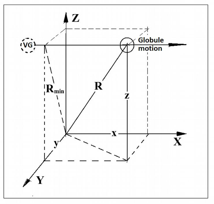
E3S Web of Conferences 196, 02001 (2020) https://doi.org/10.1051/e3sconf/202019602001
STRPEP 2020
control parameter δe f f , effective parameter of VG extension. In a general case, this equation does not
have an analytical solution and is a typical problem of linear programming.
When choosing the measure of deviation of Euclidean distance between realization and approxi-
mating function, the objective function takes the form
N
2
Φ(δ) = Fi − Mi (δ) , (5)
i=1
∂
If Mi = 0, the solution ∂δ · Φ(δ) = 0 yields a well-known least-square method. We applied a
numerical approach of search for the parameter δopt . It was determined by the minimum value of
the objective function Φ(δopt ) within the interval of possible values of the parameter δopt . For this
purpose, we used a widely used application program package MATLAB for technical and scientific
calculations. The package has Optimization Toolbox function oriented on different variants of solution
of optimization problems.
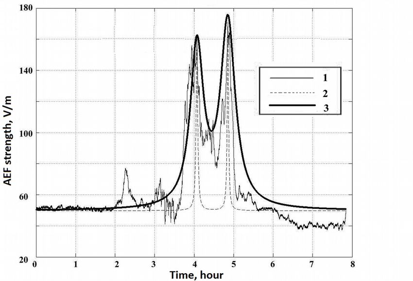
Figure 3. Response in AEF EZ during eruptive cloud passage from the explosive eruption of Shiveluch volcano
on November 16, 2014 [23] compared to the calculated curves. 1 – experimental curve; 2 – approximation by
the field of two VG point charges; 3 – approximation by the field of two VG optimizing the extension parameter
δopt =1.
As an example, we consider an explosive eruption which occurred on Shiveluch volcano at 10:17
on November 16, 2014. EC from this eruption rose up to the height of 13 km above the sea level.
Its propagation was observed on the images of Satellite Landsat 8. About two hours later, a positive
anomaly of one and a half hour long was observed in AEF Ez records at KZYG (Kozyrevsk site)
113 km to the south-west from Shiveluch volcano [24]. The anomaly looked like a double-peak bay-
like disturbance with the exceedance Ez = 125 V/m with respect to the background (Fig.3). According
to the satellite data, the time of anomaly occurrence corresponds to that of EC passage 20 km to the
east of KZYG. According to the of maximums propagation times, estimated as differences of times
between the beginning of the eruption and their arrivals, we calculated the velocities of motion for
5E3S Web of Conferences 196, 02001 (2020) https://doi.org/10.1051/e3sconf/202019602001
STRPEP 2020
two parts of the eruptive cloud as 17.7 m/s and 10.9 m/s, respectively. Agreement of aero-electric
structure propagation velocities with wind velocities (based on upper-air sounding data) at definite
heights indicates the fact that ash propagated at two horizons (9 ÷ 10 and 12 km) where temperature
inversions were observed according to upper-air sounding data.
This anomaly was approximated by the field of two VGs with point charges (curve 2, Fig.3). Then
the extension parameter δopt = 1 was optimized (curve 3, Fig.3). The latest case shows significantly
better approximation to the experimental curve.
5 Field decomposition by several globules
In most of any cases, EC electrostatic field consists of several VGs which appear as the result of
each act of magma fragmentation in volcanic conduit. Owing to the strength of applicability of the
superposition principle in this case, the resultant field Ez can be written as a sum of partial fields of
VG each of which may have its own parameters, charge sign and value as well as extension
Ez = Ak Ψ(δk ), (6)
k
The well-known law, connecting the characteristics of a separate source and the structure of the
field generated by it (1 – 3), on the basis of field character allows us to estimate charge values and
VG extension parameters responsible for recorded data formation. The most obvious algorithm of
decomposition of recorded data by dominant VG fields is the funnel algorithm for approximating
field generated by the dominant VG followed by difference series analysis.
Fig.4 illustrates VG partial field decomposition of the vertical electric field for EC from Shiv-
eluch volcano eruption on November 16, 2014. The decomposition was estimated to the level of
independence of a root-mean-square deviation relative value on iteration number. The approximation
accuracy, applying the described technique, turned to be high enough. Approximation differences
(dashed line) from the measurement data (solid line) are obvious only on the right part of Fig.4.
Figure 4. Decomposition of the vertical electric field attributed to Shiveluch volcano eruption on November 16,
2014 with respect to VG partial fields. Circle area size is proportional to VG effective size. Gray color is positive
charge, blue color is negative charge. For the background values relatively Emax , the ellipse shows the fragment
where the difference of experimental (solid line) and calculated (dashed line) data is obvious
We consider some details of application of the suggested method on the example of AEF Ez
experimental data obtained during the passage of the EC from Shiveluch volcano eruption on June
6E3S Web of Conferences 196, 02001 (2020) https://doi.org/10.1051/e3sconf/202019602001 STRPEP 2020 14, 2017 over the KLYG site (Klyuchi) [25]. In this case, ashfall ( 100 g/m3 ) was observed at the observation site located 45 km to the north from Shiveluch volcano during the passage of the EC propagating with the velocity of 4-7 km/s at the height of 12 km above the sea level. According to the paper [5], the form of a high-amplitude response in AEF EZ (-6
E3S Web of Conferences 196, 02001 (2020)                    https://doi.org/10.1051/e3sconf/202019602001
STRPEP 2020

 References
 [1] E.A. Mareev, Physics-Uspekhi, 53(5), 504–511 (2010)
 [2] E.R. Williams, "The global electrical circuit: A review", Atmospheric Research, 91, 140–152
    (2009). https://doi:10.1016/j.atmosres.2008.05.018
 [3] N.V. Krasnogorskaya, Elektrichestvo nizhnikh sloev atmosfery i metody ego izmereniya,
    (Leningrad, 1972) (in Russian)
 [4] N.V. Cherneva, P.P. Firstov, Formirovanie lokal’nogo elektricheskogo polya atmosfery na Kam-
    chatke pod vliyaniem prirodnykh protsessov [Formation of atmospheric local electric field in Kam-
    chatka under natural process effect], (Vladivostok: Dal’nauka, 2018) (in Russian)
 [5] N.V. Cherneva, E.A. Ponomarev, P.P. Firstov, A.V. Buzevich, Bulletin of KRAESC. Earth Sci-
    ences., 2:10, 60–64 (2007) (in Russian)
 [6] K. Aizawa, C. Cimarelli, M.A. Alatorre-Ibarguengoita, A. Yokoo, D. Dingwell, M. Iguchi, Earth
    and Planetary Science Letters, 444, 45–55 (2016).
 [7] S.J. Lane, M.R. James, J.S. Gilbert, Journal of Physics, Conference Series, 301(012004), 1–4
    (2011)
 [8] H. Hatakeyama, J. Meteor. Soc. Jpn., 27, 372–376 (1949) (in Japanese)
 [9] H. Hatakeyama, K. Uchikawa, J. Meteor. Soc. Jpn., 21, 84–89 (1951) (in Japanese)
 [10] S.J. Lane, J.S. Gilbert, Japan Bull., 54, 590–594 (1992)
 [11] A.W. Woods, Bull Volcanol., 50, 169–193 (1988)
 [12] M.R. James, L. Wilson, S.J. Lane, J.S. Gilbert, T.A. Mather, R.G. Harrison, R.S. Martin, Space
    Sci. Rev., 137, 399–418 (2008) DOI: 10.1007/s11214-008-9362-z
 [13] T.A. Mather, R.G. Harrison, R.S. Martin, ServGeophys, 37, 387–432 (2006)
    DOI: 10/1007/s10712-006-9007-2
 [14] S.A. Behnke, S.R. McNutt, Bull Volcanol., 76(847), 2–12 (2014) DOI: 10.1007/s00445-014-
    0847-1
 [15] A.R. Van Eaton, À. Amigo, D. Bertin et al., Geophys Res. Letters, 3563–3570 (2016)
    DOI: 10.1002/2016GL068076
 [16] R. Wall, J. Flottau, Aviation Week and Space Technology, 172, 23–25 (2010)
 [17] A.R. Van Eaton, M. Herzog, C.J.N. Wilson, J Geophys Res. Sol Ea, 117:B03203 (2012)
    https://doi:10.1029/2011JB008892
 [18] M.R.James, S.J. Lane, J.S. Gilbert, J. Geol. Soc. London, 155, 587–590 (1998)
 [19] M. Laruna, The Space Congress, Proceedings, 22–32 (1987)
 [20] T. Miura, T. Koyaguchi, Y. Tanaka, Bull Volcanol, 64, 75–93 (2002)
 [21] O.D. Kellog, Foundation of potential theory, (Berlin, 1929)
 [22] K.N. Pustovalov, P.M. Nagorskiy, Atmosphere and Ocean Optics, 29(8), 647–653 (2016)
 [23] B.P. Demidovich, I.A. Maron, Osnovy vychislitel’noy matematiki [Basis if numerical mathemat-
    ics], (Moscow, 1966) (in Russian)
 [24] P.P. Firstov, R.R. Akbashev, R. Holzworth, N. V. Cherneva, and B. M.
    Shevtsov, Izvestiya, Atmospheric and Oceanic Physics, 53(1), 24–31 (2017)
    https://doi:10.1134/10.1134/S0001433817010066
 [25] P.P. Firstov, R.R. Akbashev, N.A. Zharinov et al., Journal of Volcanology and Seismology, 13(3),
    172–184 (2019) https://doi:10.1134/S0742046319030035

                                                  8
You can also read