DEEP ACTIVE INFERENCE FOR AUTONOMOUS ROBOT NAVIGATION
←
→
Page content transcription
If your browser does not render page correctly, please read the page content below
Published as a workshop paper at “Bridging AI and Cognitive Science” (ICLR 2020)

                                        D EEP ACTIVE I NFERENCE
                                        FOR AUTONOMOUS ROBOT NAVIGATION

                                         Ozan Çatal, Samuel Wauthier, Tim Verbelen, Cedric De Boom, & Bart Dhoedt
                                         IDLab, Department of Information Technology
                                         Ghent University –imec
                                         Ghent, Belgium
                                         ozan.catal@ugent.be
arXiv:2003.03220v1 [cs.AI] 6 Mar 2020

                                                                                    A BSTRACT
                                                 Active inference is a theory that underpins the way biological agent’s perceive and
                                                 act in the real world. At its core, active inference is based on the principle that
                                                 the brain is an approximate Bayesian inference engine, building an internal gen-
                                                 erative model to drive agents towards minimal surprise. Although this theory has
                                                 shown interesting results with grounding in cognitive neuroscience, its application
                                                 remains limited to simulations with small, predefined sensor and state spaces.
                                                 In this paper, we leverage recent advances in deep learning to build more complex
                                                 generative models that can work without a predefined states space. State repre-
                                                 sentations are learned end-to-end from real-world, high-dimensional sensory data
                                                 such as camera frames. We also show that these generative models can be used to
                                                 engage in active inference. To the best of our knowledge this is the first application
                                                 of deep active inference for a real-world robot navigation task.

                                        1   I NTRODUCTION
                                        Active inference and the free energy principle underpins the way our brain – and natural agents in
                                        general – work. The core idea is that the brain entertains a (generative) model of the world which
                                        allows it to learn cause and effect and to predict future sensory observations. It does so by constantly
                                        minimising its prediction error or “surprise”, either by updating the generative model, or by inferring
                                        actions that will lead to less surprising states. As such, the brain acts as an approximate Bayesian
                                        inference engine, constantly striving for homeostasis.
                                        There is ample evidence (Friston, 2012; Friston et al., 2013a; 2014) that different regions of the brain
                                        actively engage in variational free energy minimisation. Theoretical grounds indicate that even the
                                        simplest of life forms act in a free energy minimising way (Friston, 2013).
                                        Although there is a large body of work on active inference for artificial agents (Friston et al., 2006;
                                        2009; 2017; 2013b; Cullen et al., 2018), experiments are typically done in a simulated environment
                                        with predefined and simple state and sensor spaces. Recently, research has been done on using
                                        deep neural networks as an implementation of the active inference generative model, resulting in
                                        the umbrella term “deep active inference”. However, so far all of these approaches were only tested
                                        on fairly simple, simulated environments (Ueltzhöffer, 2018; Millidge, 2019; Çatal et al., 2019). In
                                        this paper, we apply deep active inference on a robot navigation task, with high-dimensional camera
                                        observations and deploy it on a mobile robot platform. To the best of our knowledge, this is the first
                                        time that active inference is applied on a real-world robot navigation task.
                                        In the remainder of this paper we will first introduce the active inference theory in Section 2. Next,
                                        we show how we implement active inference using deep neural networks in Section 3, and discuss
                                        initial experiments in Section 4.

                                        2   ACTIVE I NFERENCE
                                        Active inference is a process theory of the brain that utilises the concept of free energy (Friston,
                                        2013) to describe the behaviour of various agents. It stipulates that all agents act in order to min-

                                                                                           1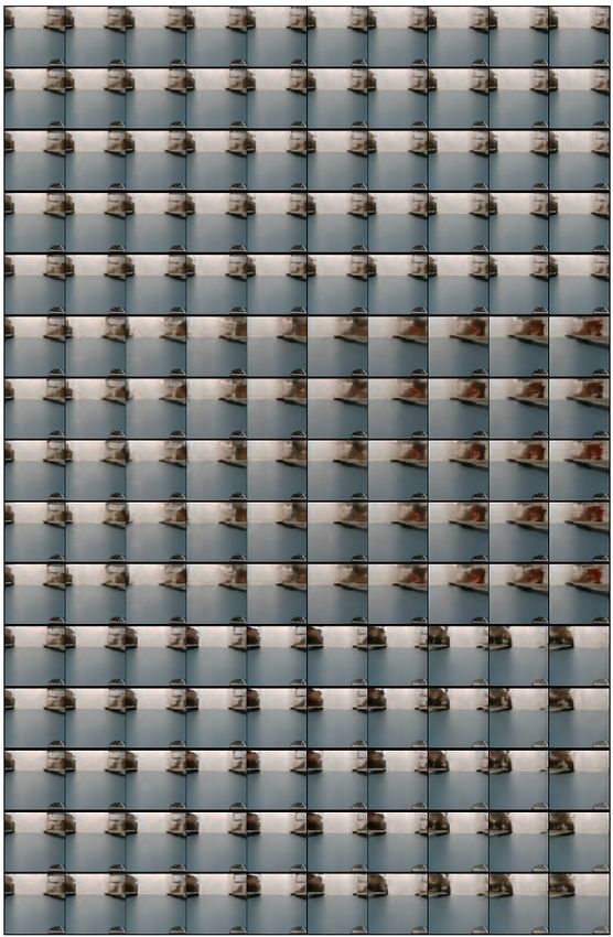
Published as a workshop paper at “Bridging AI and Cognitive Science” (ICLR 2020)

imise their own uncertainty of the world. This uncertainty is expressed as Bayesian Surprise, or
alternatively the variational free energy. In this context this is characterised by the difference be-
tween what an agent imagines about the world and what it has perceived about the world (Friston,
2010). More concretely, the agent builds a generative model P (õ, s̃, ã), linking together the agents
internal belief states s with the perceived actions a and observations o in the form of a joint distri-
bution. We use a tilde to denote a sequence of variables through time. This generative model can be
factorised as in Equation 1.
                                                        T
                                                        Y
                       P (õ, s̃, ã) = P (ã)P (s0 )         P (ot |st )P (st |st−1 , at−1 )           (1)
                                                        t=1

The free energy or Bayesian surprise is then defined as:
                             F = EQ [log Q(s̃) − log P (õ, s̃, ã)]
                               = DKL (Q(s̃)kP (s̃, ã|õ)) − log P (õ)                                 (2)
                               = DKL (Q(s̃)kP (s̃, ã)) − EQ [log P (õ|s̃)]

Here, Q(s̃) is an approximate posterior distribution. The second equality shows that free energy
is equivalent to the (negative) evidence lower bound (ELBO) (Kingma & Welling, 2013; Rezende
et al., 2014). The final equation frames the problem of free energy minimisation as explaining the
world from the agents beliefs whilst minimising the complexity of accurate explanations (Friston
et al., 2016).
Crucially, in active inference agents will act according to the belief that they will keep minimising
surprise in the future. This means agents will infer policies that yield minimal expected free energy
in the future, with a policy π being the sequence of future actions at:t+H starting at current time
step t with a time horizon H. This principle is formalised in Equation 3 with σ being the softmax
function with precision parameter γ.
                                           P (π) = σ(−γG(π))
                                                        t+H
                                                        X                                               (3)
                                           G(π) =              G(π, τ )
                                                        τ =t

Expanding the expected free energy functional G(π, τ ) we get Equation 4. Using the factorisation
of the generative model from Equation 1 we approximate Q(oτ , sτ |π) ≈ P (oτ |sτ )Q(sτ |π).
               G(π, τ ) = EQ(oτ ,sτ |π) [log Q(sτ |π) − log P (oτ , sτ |π)]
                        = EQ(oτ ,sτ |π) [log Q(sτ |π) − log P (oτ |sτ , π) − log P (sτ |π)]             (4)
                        = DKL (Q(sτ |π)kP (sτ )) + EQ(sτ ) [H(P (oτ |sτ ))]

Note that, in the final equality, we substitute P (sτ |π) by P (sτ ), a global prior distribution on the so-
called “preferred” states of the agent. This reflects the fact that the agent has prior expectations about
the states it will reach. Hence, minimising expected free energy entails both realising preferences,
while minimising the ambiguity of the visited states.

3    D EEP ACTIVE INFERENCE
In current treatments of active inference the state spaces are typically completely fixed upfront (Fris-
ton et al., 2009; Millidge, 2019) or partially (Ueltzhöffer, 2018). However, this does not scale well
for more complex tasks as it is often difficult to design meaningful state spaces for such problems.
Therefore we allow for the agent to learn by itself what the exact parameterisation of its belief
space should be. We enable this by using deep neural networks to generate the various necessary
probability distributions for our agent.
We approximate the variational posterior distribution for a single timestep Q(st |st−1 , at−1 , ot ) with
a network qφ (st |st−1 , at−1 , ot ). Similarly we approximate the likelihood model P (ot |st ) with the
network pξ (ot |st ) and the prior P (st |st−1 , at−1 ) with the network pθ (st |st−1 , at−1 ). Each of

                                                         2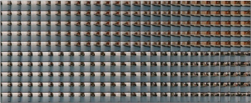
Published as a workshop paper at “Bridging AI and Cognitive Science” (ICLR 2020)

Figure 1: The various components of the agent rolled out trough time. We minimise the variational
free energy by minimising both the negative log likelihood of observations and the KL divergence
between the state transition model and the observation model. The inferred hidden state is charac-
terised as a multivariate Gaussian distribution.

the networks output a multivariate normal distribution with a diagonal covariance matrix using the
reparameterisation trick (Kingma & Welling, 2013). These neural networks cooperate in a way
similar to a VAE, where the fixed standard normal prior is replaced with the learnable prior pθ , the
decoder by pξ and finally the encoder by qφ , as visualised in Figure 1.
These networks are trained end-to-end using the free energy formula from the previous section as
an objective.
        ∀t : minimise : − log pξ (ot |st ) + DKL (qφ (st |st−1 , at−1 , ot )kpθ (st |st−1 , at−1 )) (5)
               φ,θ,ξ

As in a conventional VAE (Kingma & Welling, 2013) the negative log likelihood (NLL) term in the
objective punishes reconstruction error forcing the model to learn relevant information on the belief
state to be captured in the posterior output, while the KL term pulls the prior output towards the
posterior output, forcing the prior and posterior to agree on the content of the belief state in a way
that still allows the likelihood model to reconstruct the current observation.
We can now use the learned models to engage in active inference, and infer which action the agent
has to take next. This is done by generating imagined trajectories for different policies using pθ
and pξ , calculating the expected free energy G and selecting the action of the policy that yields the
lowest G. These policies to evaluate can be predefined, or generated through random shooting, using
cross-entropy method (Boer et al., 2005) or by building a search tree.

4   E XPERIMENTS
We validate our deep active inference approach on a real world robotics navigation task. First, we
collect a dataset consisting of two hours worth of real world action-observation sequences by driving
a Kuka Youbot base platform up and down the aisles of a warehouse lab. Camera observations are
recorded with a front mounted Intel Realsense RGB-D camera, without taking into account the
depth information. The x, y and angular velocities are recorded as actions at a recording frequency
of 10Hz. The models are trained on a subsampled version of the data resulting in a train set with
data points every 200ms.
Next, we instantiate neural networks qφ and pξ as a convolutional encoder and decoder network,
and pθ using an LSTM. These are trained with Adam optimizer using the objective function from
Equation 5 for 1M iterations. We use a minibatch size of 128 and a sequence length of 10 timesteps.
A detailed overview of all hyperparameters is given in appendix.
We utilise the same approach as in Çatal et al. (2020) for our imaginary trajectories and planning.
The agent has access to three base policies to pick from: drive straight, turn left and turn right. Ac-
tions from these policies are propagated to the learned models at different time horizons H = 10, 25

                                                  3
Published as a workshop paper at “Bridging AI and Cognitive Science” (ICLR 2020)
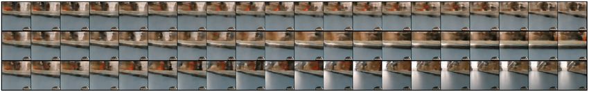
(a) Preferred state. (b) Start state
(c) Imaginary future trajectories for different policies, i.e. going straight ahead (top), turning right (middle),
turning left (bottom).
(d) Actually followed trajectory.
Figure 2: Experimental results: Figure (a) shows the target observation in imagined (reconstructed)
space. (b) The start observation of the trial. Figure (c) shows different imaginary planning results,
whilst (d) shows the actually followed trajectory.
or 55. For each resulting imaginary trajectory, the expected free energy G is calculated. Finally the
trajectory with lowest G is picked, and the first action of the chosen policy is executed, after which
the imaginary planning restarts. The robot’s preferences are given by demonstration, using the state
distribution of the robot while driving in the middle of the aisle. This should encourage the robot to
navigate in the aisles.
At each trial the robot is placed at a random starting position and random orientation and tasked
to navigate to the preferred position. Figure 2 presents a single experiment as an illustrative exam-
ple. Figure 2a shows the reconstructed preferred observation from the given preferred state, while
Figure 2b shows the trial’s start state from an actual observation. Figure 2c shows the imagined
results of either following the policy “always turn right”, “always go straight” or “always turn left”.
Figure 2d is the result of utilising the planning method explained above. Additional examples can
be found in the supplementary material.
The robot indeed turns and keeps driving in the middle of the aisle, until it reaches the end and then
turns around 1 . When one perturbs the robot by pushing it, it will again recover and continue to the
middle of the aisle.
5 C ONCLUSION
In this paper we present how we can implement a generative model for active inference using deep
neural networks. We show that we are able to successfully execute a simple navigation task on a
real world robot with our approach. As future work we want to allow the robot to continuously learn
from past autonomous behaviour, effectively “filling the gaps” in its generative model. Also how
1
A movie demonstrating the results is available at https://tinyurl.com/smvyk53
4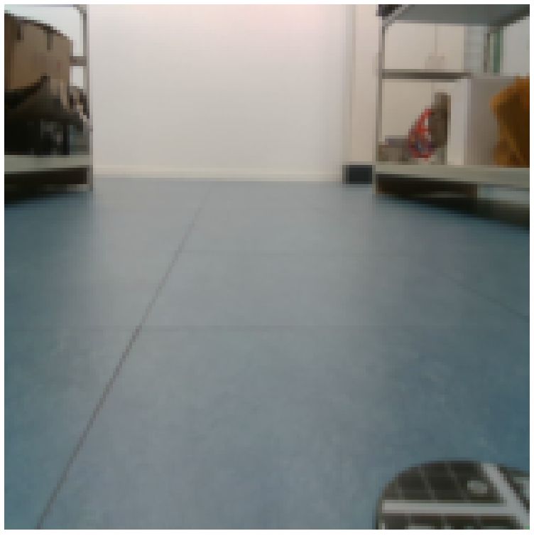
Published as a workshop paper at “Bridging AI and Cognitive Science” (ICLR 2020)

to define the “preferred state” distributions and which policies to evaluate remains an open research
challenge for more complex tasks and environments.

R EFERENCES
Pieter-Tjerk Boer, Dirk Kroese, Shie Mannor, and Reuven Rubinstein. A tutorial on the cross-
  entropy method. Annals of Operations Research, 134:19–67, 02 2005. doi: 10.1007/
  s10479-005-5724-z.

Ozan Çatal, Johannes Nauta, Tim Verbelen, Pieter Simoens, and Bart Dhoedt. Bayesian policy
  selection using active inference. In Workshop on Structure & Priors in Reinforcement Learning
  at ICLR 2019 : proceedings, pp. 9, 2019.

Ozan Çatal, Tim Verbelen, Johannes Nauta, Cedric De Boom, and Bart Dhoedt. Learning perception
  and planning with deep active inference. In IEEE International Conference on Acoustics, Speech
  and Signal Processing, ICASSP, Barcelona, Spain, pp. In Press, 2020.

Maell Cullen, Ben Davey, Karl J. Friston, and Rosalyn J. Moran. Active inference in openai gym:
 A paradigm forcomputational investigations into psychiatricillness. Biological Psychiatry: Cog-
 nitive Neuroscience and Neuroimaging, 3(9):809 – 818, 2018. ISSN 2451-9022. doi: https://doi.
 org/10.1016/j.bpsc.2018.06.010. URL http://www.sciencedirect.com/science/
 article/pii/S2451902218301617. Computational Methods and Modeling in Psychi-
 atry.

Karl Friston. The free-energy principle: A unified brain theory? Nature Reviews Neuroscience, 11
  (2):127–138, 2010. ISSN 1471003X. doi: 10.1038/nrn2787. URL http://dx.doi.org/
  10.1038/nrn2787.

Karl Friston. A free energy principle for biological systems. Entropy, 14(11):2100–2121, 2012.
  ISSN 1099-4300. doi: 10.3390/e14112100. URL https://www.mdpi.com/1099-4300/
  14/11/2100.

Karl Friston, James Kilner, and Lee Harrison. A free energy principle for the brain. Journal of
  Physiology Paris, 100(1-3):70–87, 2006. ISSN 09284257. doi: 10.1016/j.jphysparis.2006.10.001.

Karl Friston, Philipp Schwartenbeck, Thomas Fitzgerald, Michael Moutoussis, Tim Behrens, and
  Raymond Dolan. The anatomy of choice: active inference and agency. Frontiers in Human
  Neuroscience, 7:598, 2013a. ISSN 1662-5161. doi: 10.3389/fnhum.2013.00598. URL https:
  //www.frontiersin.org/article/10.3389/fnhum.2013.00598.

Karl Friston, Philipp Schwartenbeck, Thomas FitzGerald, Michael Moutoussis, Timothy Behrens,
  and Raymond J. Dolan. The anatomy of choice: active inference and agency. Fron-
  tiers in Human Neuroscience, 7(September):1–18, 2013b. ISSN 1662-5161. doi: 10.3389/
  fnhum.2013.00598. URL http://journal.frontiersin.org/article/10.3389/
  fnhum.2013.00598/abstract.

Karl Friston, Thomas FitzGerald, Francesco Rigoli, Philipp Schwartenbeck, John O’Doherty,
  and Giovanni Pezzulo. Active inference and learning. Neuroscience & Biobehavioral Re-
  views, 68:862 – 879, 2016. ISSN 0149-7634. doi: https://doi.org/10.1016/j.neubiorev.
  2016.06.022. URL http://www.sciencedirect.com/science/article/pii/
  S0149763416301336.

Karl Friston, Thomas FitzGerald, Francesco Rigoli, Philipp Schwartenbeck, and Giovanni Pezzulo.
  Active inference: A Process Theory. Neural Computation, 29:1–49, 2017. ISSN 1530888X. doi:
  10.1162/NECO a 00912.

Karl J Friston. Life as we know it. Journal of the Royal Society Interface, 2013.

Karl J. Friston, Jean Daunizeau, and Stefan J. Kiebel. Reinforcement learning or active inference?
  PLOS ONE, 4(7):1–13, 07 2009. doi: 10.1371/journal.pone.0006421. URL https://doi.
  org/10.1371/journal.pone.0006421.

                                                 5
Published as a workshop paper at “Bridging AI and Cognitive Science” (ICLR 2020)

Karl J Friston, Philipp Schwartenbeck, Thomas F. Fitzgerald, Michael Moutoussis, Timothy W.
  Behrens, and Raymond J. Dolan. The anatomy of choice: dopamine and decision-making. In
  Philosophical Transactions of the Royal Society B: Biological Sciences, 2014.
Diederik P. Kingma and Max Welling. Auto-encoding variational bayes. CoRR, abs/1312.6114,
  2013. URL http://arxiv.org/abs/1312.6114.
Beren Millidge. Deep active inference as variational policy gradients. CoRR, abs/1907.03876, 2019.
  URL http://arxiv.org/abs/1907.03876.
Danilo Jimenez Rezende, Shakir Mohamed, and Daan Wierstra. Stochastic backpropagation and
  approximate inference in deep generative models. In Eric P. Xing and Tony Jebara (eds.), Pro-
  ceedings of the 31st International Conference on Machine Learning, volume 32 of Proceedings
  of Machine Learning Research, pp. 1278–1286, Bejing, China, 22–24 Jun 2014. PMLR. URL
  http://proceedings.mlr.press/v32/rezende14.html.
Kai Ueltzhöffer. Deep active inference. Biological Cybernetics, 112(6):547–573, Dec 2018.
  ISSN 1432-0770. doi: 10.1007/s00422-018-0785-7. URL https://doi.org/10.1007/
  s00422-018-0785-7.

                                                6
Published as a workshop paper at “Bridging AI and Cognitive Science” (ICLR 2020)
Supplementary Material
A N EURAL ARCHITECTURE
Layer Neurons/Filters activation function
Convolutional 8 Leaky ReLU
Convolutional 16 Leaky ReLU
Posterior Convolutional 32 Leaky ReLU
Convolutional 64 Leaky ReLU
Convolutional 128 Leaky ReLU
Concat N.A. N.A.
Linear 2 x 128 states Softplus
Linear 128 x 8 x 8 Leaky ReLU
Likelihood
Convolutional 128 Leaky ReLU
Convolutional 64 Leaky ReLU
Convolutional 32 Leaky ReLU
Convolutional 16 Leaky ReLU
Convolutional 8 LeakyReLU
LSTM cell 400 Leaky ReLU
Prior
Linear 2 x128 states Softplus
Table 1: Neural network architectures. All convolutional layers have a 3x3 kernel. The convolutional
layers in the Likelihood model have a stride and padding of 1 to ensure that they preserve the input
shape. Upsampling is done by nearest neighbour interpolation. The concat step concatenates the
processed image pipeline with the vector inputs a and s.
7Published as a workshop paper at “Bridging AI and Cognitive Science” (ICLR 2020)
B H YPERPARAMETERS
Parameter Value
learning rate 0.0001
Learning
batch size 128
train iterations 1M
sequence length 10
γ 100
Planning
D (Çatal et al., 2020) 1
K (Çatal et al., 2020) 10, 25, 55
N (Çatal et al., 2020) 5
ρ (Çatal et al., 2020) 0.001
Table 2: Overview of the model hyperparemeters.
8Published as a workshop paper at “Bridging AI and Cognitive Science” (ICLR 2020)
C D ETAILED P LANNING EXAMPLE
A movie demonstrating the results is available at https://tinyurl.com/smvyk53.
Figure 3: Trial preferred state
9Published as a workshop paper at “Bridging AI and Cognitive Science” (ICLR 2020)
Figure 4: Short term planning
10Published as a workshop paper at “Bridging AI and Cognitive Science” (ICLR 2020)
Figure 5: Middle long term planning
11Published as a workshop paper at “Bridging AI and Cognitive Science” (ICLR 2020)
Figure 6: Long term planning
12You can also read