TUC MEDIA COMPUTING AT BIRDCLEF 2021: NOISE AUGMENTATION STRATEGIES IN BIRD SOUND CLASSIFICATION IN COMBINATION WITH DENSENETS AND RESNETS

TUC Media Computing at BirdCLEF 2021: Noise
augmentation strategies in bird sound classification
in combination with DenseNets and ResNets
Arunodhayan Sampathkumar1 , Danny Kowerko1
1
 Technische Universität Chemnitz, Str. der Nationen 62, 09111 Chemnitz

 Abstract
 This research paper presents deep learning techniques for bird recognition to classify 397 species in the
 BirdCLEF 2021 challenge. The proposed method was inspired by the DCASE2019 audio tagging chal-
 lenge, which classifies and recognizes different sound events. Data augmentations methods like noise
 augmentation, spectrogram augmentation techniques are used to avoid overfitting and hence generalize
 the model. The final solution is based on an ensemble of different backbone models and splitting the
 dataset based on geographic locations provided in the test set. Furthermore, framewise post-processing
 predictions are used to identify the bird events. The best results were obtained from 12 model ensembles
 with a public and private score of 0.6487 and 0.6034, respectively.

 Keywords
 CNN (Convolutional Neural Network), Bird Recognition, Deep learning, Data Augmentation, Sound-
 scapes

1. Introduction
Manual monitoring of birds species requires lots of human labor and is difficult in many forest
areas. An automated approach in an ecosystem for continuous recordings would allow moni-
toring species in different locations, over longer period of time, and in deeper forest areas [1].
In 2021, BirdCLEF has organized a challenge to classify 397 bird species in 5-300 s snippets of
continuous audio recordings in different location around the globe. The test data contain 80
soundscapes recording each of 10 minutes length, recorded in 4 different locations namely COL
(Jardín, Departamento de Antioquia, Colombia), COR (Alajuela, San Ramón, Costa Rica), SNE
(Sierra Nevada, California, USA), SSW(Ithaca, New York, USA)[2, 3]. The soundscape recordings
contain high quality overlapping sounds of different species. A challenging part and motivation
of the competition are the weakly labeled train data, and there are multiple distribution domain
shifts present, namely shifts in input space, shifts in prior probability of labels, and shifts in the
function which connects train and test recordings. Domain shifts in this competition are large
differences in data characteristics between train (clean recordings) and test (noisy recordings)
making generalization of models on unseen data difficult.

CLEF 2021 – Conference and Labs of the Evaluation Forum, September 21–24, 2021, Bucharest, Romania
" arunodhayan.sampath-kumar@informatik.tu-chemnitz.de (A. Sampathkumar);
danny.kowerko@informatik.tu-chemnitz.de (D. Kowerko)
 © 2021 Copyright for this paper by its authors. Use permitted under Creative Commons License Attribution 4.0 International (CC BY 4.0).
 CEUR
 Workshop
 Proceedings
 http://ceur-ws.org
 ISSN 1613-0073 CEUR Workshop Proceedings (CEUR-WS.org)

The paper is organized as follows, section 2 describes the recognition of the birds includ-
ing data preparation. Section 3 describes feature extraction, data-augmentation, neural network
architecture and training steps. Section 4 presents the evaluation results followed by the
conclusion.

2. Dataset
All the recordings are first converted from ogg to wav format with a sampling rate of 32 kHz.
The soundscape recordings are prepared for validation by cutting them into 5 s chunks according
to the annotations. The background noises are separated from the soundscape recordings based
on parts without bird activity using the provided metadata. Later, these background noises are
used for data augmentation.
Some parts of validation soundscape recordings are merged with Xeno-canto training set [3]
for training, while the rest of the recordings are used for cross validation. The training set and
validation set are splitted by 5 stratified folds.
To create more diverse models, 6 different sub-datasets are formed targeting different locations,
which are later ensembeled.

Table 1
The Table illustrates the description of the datasets.
 ID No of Classes No of training Location Radius
 samples (km)
 Dataset-1 273 47168 United states, Costa Rica 200
 Colombia
 Dataset-2 345 57302 United states, Costa Rica 400
 Colombia
 Dataset-3 391 32963 United states, Costa Rica -
 Colombia
 Dataset-4 263 44913 United states -
 Dataset-5 162 25760 Costa Rica -
 Dataset-6 187 29831 Colombia -

 As presented in Table 1, sub-datasets are divided based on locations, e.g. Dataset-1 and 2
are prepared based on the locations of test set. With the given latitude and longitude from test
data, a 200 and 400 km radius is marked and most likely occurring species within the radius are
taken into account.
Dataset-3 consist of species that mainly occur in the given test recording locations. Dataset-4
belongs to species that mainly present in the recording locations of the United States. Dataset-5
belongs to species that mainly present in the recording locations of Costa Rica. Dataset 6
belongs to species that mainly present in the recording locations of Colombia.

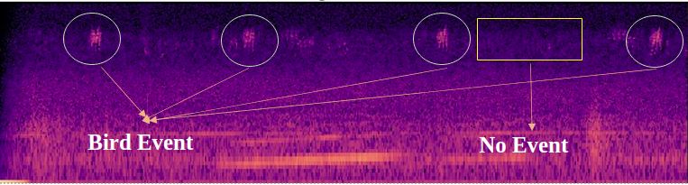
3. Methodology
3.1. Spectrogram Extraction
The recordings are sampled at 32 kHz sample rate and trimmed to 30 s long chunks because
if we use a shorter window size, it may not include any sound events or include some sound
events which may be a noisy event or a background species as shown in Figure 1, for this reason
longer chunks are preferred. To make the model learn correctly, we need to make each label
correspond to call-events of each species. First, we compute a Short Time Fourier Transform
(STFT) with a Hann window of 1024 samples and hop size of 384 samples and mel bins of 64,
retain only the magnitude and then followed by applying a log-mel filter banks from 150 Hz to
15 kHz.

Figure 1: The figure presents a log-mel spectrogram, where 30 s long chunk window represents many
bird events, whereas a random 5 s short (from 20 s-25 s) chunk window represents no event

3.2. DataAugmentation
Different data augmentation techniques are performed to increase the model performance and
improve its generalization to real time data. The following data augmentation methods are
applied to raw audio recordings:

 • 30 s chunk at random position for training
 • Gaussian Noise
 • Gaussian Signal to Noise Ratio (SNR)
 • Adding primary background noise
 • Adding secondary background noise
 • Mixup augmentation
 • Spectrogram augmentation

Primary background noise: The train recordings and test recordings contain domain shifts.
To make train recordings more robust, different noises are incorporated as background noise.
Besides the noise extracted from soundscape recordings, recordings without bird activity from
BAD (Bird Audio Detection) are used [4]. Apart from these two noise systems, generated pink
noises are used [5].

Secondary background noise: Mixing various (bursts of overlapping) short audios in the
train recording with random pauses between. Noises like wind, car sounds, insects, rain and
thunder are used.
Mixup: Audio chunks from random files are mixed together, and their corresponding labels are
added as shown in Figure 2. The mixup augmentations are constructed using the formulae [6].

 = · + (1 − ) · (1)
 = · + (1 − ) · (2)
 where ( , ) and ( , ) are the two randomly selected recordings for mixup, and is the
mix ratio with values from [0, 1]. Mixup increases the robustness of the model and generalizes
well in real time data because soundscape data typically contain more than one species occurring
in the event window.

Figure 2: The top left indicates the spectrogram of species acafly and top right indicates brewee. The
bottom spectrogram indicates the mixup of acafly and brewee

 Gaussian SNR: The Gaussian noise applied to the samples with random signal to Noise
Ratio (SNR).
Spectrogram augmentation Time stretching and pitch shifting are the augmentations tried
on spectrograms. Time stretching is the process of changing the speed/duration of sound
without affecting the pitch of sound. It takes the wave samples and a factor by which the input is
stretched by a factor of 0.4 which has a small difference with the original sample. Pitch shifting
is the process of changing the pitch of the sound without affecting the speed. It takes wave
samples, sample rate and number of steps(-4 to +4) through which the pitch must be shifted.
These methods are performed using LIBROSA library [7, 8].

Table 2
Influence of data augmentations on the model results. The backbone architecture used here is
DenseNet 161.
 ID Description F1 score
 1 Baseline, no augmentation 0.58
 2 Baseline with noisy recordings extracted from soundscapes 0.60
 (primary background noise)
 3 Baseline with noisy recordings extracted from soundscapes 0.61
 (primary background noise) + secondary background noise BAD
 4 Baseline with BAD 0.62
 (primary background noise) + secondary background noise BAD
 5 Baseline with BAD as primary + secondary background noise noisy 0.615
 soundscapes
 6 Baseline with BAD as primary + secondary background noise pink 0.595
 noise
 7 Baseline with noisy recordings extracted from soundscapes 0.64
 (primary background noise) + secondary background noise
 (wind,car,rain noises)+BAD+ spec augmentation

3.3. Network Architecture
In recent years Convolutional Neural Networks (CNNs) have been successfully used for audio
recognition and detection. The architecture design for the bird recognition task was inspired
from DCASE2019 PANNs (Large-Scale Pretrained Audio Neural Networks for Audio Pattern
Recognition) [7]. PANNs are developed based on cross talk CNN with an extra fully connected
layer added to the penultimate layer of the CNN.
From the previous BirdCLEF challenges, deeper CNN networks performed well when compared
with wider or shallow CNNs. Hence the backbone network for this challenge used are ResNets
[9] and DenseNets [10].

 ResNet: Deeper CNNs perform well on audio recognition tasks. The challenge in very deep
CNNs is that the gradients do not propagate properly. To solve this issue, ResNets introduced
shortcut connections between convolutional layers.

 DenseNets: DenseNets were designed to improve the information flow between layers, a
different connectivity pattern was introduced with direct connections from any layer to all
subsequent layers. The change of feature maps is facilitated by down-sampling the architecture
by dividing the network into multiple densely connections, making the network deeper.

 In this task, after log-mel feature extraction, the inputs are passed to ResNets/DenseNets
by removing the last fully connected layers and extract only features. Then, a modified 1D
attention based fully connected layer is attached to ResNet. The output of this network is a
dictionary which contains clipwise and framewise outputs. Table 3 illustrates the modified
networks used in this research.

Table 3
Configuration of ResNet 50 and DenseNets used here for bird recognition.
 ResNet 50 DenseNet121 DenseNet161
 Log mel spectrogram 1024 Log mel spectrogram 1024 Log mel spectrogram 1024
 window size x 64 mel bins window size x 64 mel bins window size x 64 mel bins
 ResNet-50 features DenseNet-121 features DenseNet-161 features
 Maxpooling 1D Maxpooling 1D Maxpooling 1D
 AveragePooling 1D AveragePooling 1D AveragePooling 1D
 Merge Merge Merge
 Maxpooling+Average Pool- Maxpooling+Average Pool- Maxpooling+Average Pool-
 ing ing ing
 Fully connected layer+ReLu Fully connected layer+ReLu Fully connected layer+ReLu
 Attention 1D+ no of Attention 1D+ no of Attention 1D+ no of
 classes+Sigmoid classes+Sigmoid classes+Sigmoid
 Framewise output Framewise output Framewise output
 Clipwise output Clipwise output Clipwise output

3.4. Training setup
Our CNNs used a model pretrained on ImageNet [7], and were fine-tuned with training data
previously converted to log-mel scaled spectrogram images. Machine learning functionality
was implemented using the PyTorch library, while audio (pre-)processing functionality like
spectrogram decomposition was realized using the Librosa library.
 The networks are trained for 75 epochs without mixup augmentation and 150 epochs with
mixup augmentation. The loss function used here is BCE-focal-2way loss (binary cross entropy)
and sed- scaled-pos-neg-focalloss(FL) [11].
SED-Scaled-Pos-Neg-Focal loss: It focuses on primary labels and secondary labels loss.

 = ( , ℎ) (3)

 − − = (1 − ( )) · (1 − ) · (4)
 − − = ( ) · (1 − ) · (5)
 = (4) + (5) (6)
 = ( > 0.0, − , − ) (7)
 − = · (8)
 Oneslike are tensors filled with the scalar value ‘1‘and zerolike are tensors filled with the
scalar value ‘0‘.
The grouped output losses are Focalloss-scaled, bceloss, Focalloss.
The optimizer used here is AdamW optimizer with weight decay 0.1. The learning rate scheduler
is a combination of merging Cosine Annealing Scheduler with warmup (cycle-size is epoch-
length number of epochs) + LinearCyclicalScheduler (cycle-size is epoch-length 
2). The initial learning rate is 0.001. Background species metadata are not taken into account.

4. Evaluation results
This section illustrates the combination of models, ensemble techniques and evaluation score
on the test set. Table 4, Table 5, and Table 6 illustrate the different strategies used in the model
and their respective results based on public and private leadership board. The ensemble method
used here is voting.

Table 4
Illustration of Dense161 models used for submissions. NS denotes Noisy Soundscapes.
 Model ID M1 M2 M3 M4 M5 M6 M7 M8
 Ensemble RUN 1 1,4 2,4 2,4 2 3,4 3,4 3,4
 Network Type Dense161 Dense161 Dense161 Dense161 Dense161 Dense161 Dense161 Dense161
 Chunk duration[s] 30 30 30 30 30 30 30 30
 No of Classes 397 397 391 343 273 162 187 263
 Primary BAD NS NS NS NS NS NS NS
 Background noise
 Secondary BAD NS BAD+ BAD+ BAD+ BAD+ BAD+ BAD+
 Background noise other other other other other other
 noises noises noises noises noises noises
 OtherAugmentations yes yes yes yes yes yes yes yes
 Public Score 0.5981 0.6134 0.6013 0.6214 0.6298 - - -
 Private Score 0.5638 0.5789 0.5609 0.5822 0.5899 - - -

Table 5
Illustration of Dense121 models used for submissions. NS denotes Noisy Soundscapes.
 Model ID M9 M10 M11 M12 M13
 Ensemble RUN 1 ,4 2,4 2,4 2
 Network Type Dense121 Dense121 Dense121 Dense121 Dense121
 Chunk duration[s] 30 30 30 30 30
 No of Classes 397 397 391 343 273
 Primary BAD NS NS NS NS
 Background noise
 Secondary BAD NS BAD+ BAD+ BAD+
 Background noise other other other
 noises noises noises
 OtherAugmentations yes yes yes yes yes
 Public Score 0.5800 0.5949 0.5866 0.6033 0.6046
 Private Score 0.5598 0.5698 0.5587 0.5789 0.5699

Table 6
Illustration of ResNet50 models used for submissions. NS denotes Noisy Soundscapes.
 Model ID M14 M15 M16 M17 M18
 Ensemble RUN 1 1,4 2,4 2,4 2
 Network Type ResNet50 ResNet50 ResNet50 ResNet50 ResNet50
 Chunk duration[s] 30 30 30 30 30
 No of Classes 397 397 391 343 273
 Primary BAD NS NS NS NS
 Background noise
 Secondary BAD NS BAD+ BAD+ BAD+
 Background noise other other other
 noises noises noises
 OtherAugmentations yes yes yes yes yes
 Public Score 0.5914 0.6089 0.6088 0.6366 0.6277
 Private Score 0.56878 0.5677 0.5789 0.5977 0.5989

 Ensemble RUN 1: Models M1, M2, M9, M10, M14, and M15 are used. This model contains
397 classes and used different background noises. The clipwise threshold, framewise threshold
and number of votes are discussed in the table 7.

Table 7
The table illustrates different voting strategies and thresholds their respective scores
 6 Models Clipwise Framewise Public score Private
 Threshold Threshold score
 3 Votes 0.3 0.3 0.6466 0.5993
 3 Votes 0.5 0.5 0.6502 0.5989
 4 Votes 0.3 0.3 0.6314 0.5891
 4 Votes 0.5 0.5 0.6389 0.5904

Ensemble RUN 2: Models M3, M4, M5, M11, M12, M13, M16, M17, and M18 are used. This
model contains 391, 345 and 273 classes, and used different background noises. The clipwise
threshold, framewise threshold and number of votes are discussed in the table 8. The 9 model
ensemble is a combination of different classes which are split based on location and achieved
the top score of 0.6741 in our public score with less False Positives and 0.6024 in the private
score.

Table 8
The table illustrates different voting strategies and thresholds their respective scores
 9 Models Clipwise Framewise Public score Private
 Threshold Threshold score
 4 Votes 0.3 0.3 0.6436 0.6024
 4 Votes 0.5 0.5 0.6474 0.6007
 3 Votes 0.3 0.3 0.67741 0.5988
 3 Votes 0.5 0.5 0.6741 0.5899

Ensemble RUN 3: Models M7, M8, and M9 are used. This model contains 162, 187 and
263 classes and used different background noises. The clipwise threshold, framewise threshold
and number of votes are discussed in the table 9. This ensemble method comprises of 3 different
locations. The 3 model ensemble based on location split has a score of 0.6799 on public score
with less FP compared to 0.5951 on private score.
 Ensemble RUN 4: Models M2, M3, M4, M6, M7, M8, M10, M11, M12, M15, M16, and M17 are

Table 9
The table illustrates different voting strategies and thresholds their respective scores
 9 Models Clipwise Framewise Public score Private
 Threshold Threshold score
 1 Vote 0.3 0.3 0.6799 0.5951
 1 Vote 0.5 0.5 0.6743 0.5823

used. This RUN takes best performing models which used different background noises. The
clipwise threshold, framewise threshold and number of votes are discussed in Table 10. This
ensemble method comprises of 12 different models with different backbone models and different
classes split based on location yields the best private score of 0.6034.

Table 10
The table illustrates different voting strategies, thresholds, and their respective scores
 12 Models Clipwise Framewise Public score Private
 Threshold Threshold score
 5 Votes 0.3 0.3 0.6487 0.6034
 5 Votes 0.5 0.5 0.6484 0.6030
 6 Votes 0.3 0.3 0.6474 0.6024
 6 Votes 0.5 0.5 0.6453 0.6013

5. Conclusion and Future Work
The current approach attained an F1 score of 0.6034 in the private leadership board. Recognizing
all bird species is still challenging because of domain shift in train (clean audio) and test (noisy
audio) data. The train dataset consists of weakly labeled (clipwise labeling) and there were many
background species present. A multi-label annotation of train files could have significantly
improved the models in bird recognition.
There are several techniques to improve this bird recognition task, methods like vision trans-
forms and removal of no bird activity from the train dataset. A promising approach would be
the feature extraction by merging two different features in combination with polyphonic event
detection. Better inference techniques could focus more on locations, e.g. using the ebird API
and thresholds for each species separately, to achieve better recognition of bird events.

References
 [1] M. Mühling, J. Franz, N. Korfhage, B. Freisleben, Bird species recognition via neural
 architecture search, in: L. Cappellato, C. Eickhoff, N. Ferro, A. Névéol (Eds.), Working
 Notes of CLEF 2020 - Conference and Labs of the Evaluation Forum, Thessaloniki, Greece,
 September 22-25, 2020, volume 2696 of CEUR Workshop Proceedings, CEUR-WS.org, 2020.
 URL: http://ceur-ws.org/Vol-2696/paper_188.pdf.
 [2] A. Joly, H. Goëau, S. Kahl, L. Picek, T. Lorieul, E. Cole, B. Deneu, M. Servajean, R. Ruiz De
 Castañeda, I. Bolon, H. Glotin, R. Planqué, W.-P. Vellinga, A. Dorso, H. Klinck, T. Denton,
 I. Eggel, P. Bonnet, H. Müller, Overview of lifeclef 2021: a system-oriented evaluation of
 automated species identification and species distribution prediction, in: Proceedings of
 the Twelfth International Conference of the CLEF Association (CLEF 2021), 2021.
 [3] S. Kahl, T. Denton, H. Klinck, H. Glotin, H. Goëau, W.-P. Vellinga, R. Planqué, A. Joly,
 Overview of birdclef 2021: Bird call identification in soundscape recordings, in: Working
 Notes of CLEF 2021 - Conference and Labs of the Evaluation Forum, 2021.
 [4] V. Lostanlen, J. Salamon, A. Farnsworth, S. Kelling, J. P. Bello, Birdvox-full-night: A dataset
 and benchmark for avian flight call detection, in: 2018 IEEE International Conference
 on Acoustics, Speech and Signal Processing, ICASSP 2018, Calgary, AB, Canada, April
 15-20, 2018, IEEE, 2018, pp. 266–270. URL: https://doi.org/10.1109/ICASSP.2018.8461410.
 doi:10.1109/ICASSP.2018.8461410.
 [5] J. O. Smith, Spectral Audio Signal Processing, http://ccrma.stanford.edu/jos/-
 sasp/, accessed . Online book, 2011 edition.
 [6] K. Xu, D. Feng, H. Mi, B. Zhu, D. Wang, L. Zhang, H. Cai, S. Liu, Mixup-based acous-
 tic scene classification using multi-channel convolutional neural network, in: R. Hong,
 W. Cheng, T. Yamasaki, M. Wang, C. Ngo (Eds.), Advances in Multimedia Information
 Processing - PCM 2018 - 19th Pacific-Rim Conference on Multimedia, Hefei, China,
 September 21-22, 2018, Proceedings, Part III, volume 11166 of Lecture Notes in Com-
 puter Science, Springer, 2018, pp. 14–23. URL: https://doi.org/10.1007/978-3-030-00764-5_2.
 doi:10.1007/978-3-030-00764-5\_2.
 [7] Q. Kong, Y. Cao, T. Iqbal, Y. Wang, W. Wang, M. D. Plumbley, Panns: Large-scale pretrained
 audio neural networks for audio pattern recognition, CoRR abs/1912.10211 (2019). URL:
 http://arxiv.org/abs/1912.10211. arXiv:1912.10211.
 [8] B. McFee, C. Raffel, D. Liang, D. P. Ellis, M. McVicar, E. Battenberg, O. Nieto, librosa:
 Audio and music signal analysis in python, in: Proceedings of the 14th python in science
 conference, volume 8, 2015.
 [9] H. Zhang, C. Wu, Z. Zhang, Y. Zhu, Z. Zhang, H. Lin, Y. Sun, T. He, J. Mueller, R. Manmatha,
 M. Li, A. J. Smola, Resnest: Split-attention networks, CoRR abs/2004.08955 (2020). URL:
 https://arxiv.org/abs/2004.08955. arXiv:2004.08955.
[10] G. Huang, Z. Liu, K. Q. Weinberger, Densely connected convolutional networks, CoRR
 abs/1608.06993 (2016). URL: http://arxiv.org/abs/1608.06993. arXiv:1608.06993.
[11] T. Lin, P. Goyal, R. B. Girshick, K. He, P. Dollár, Focal loss for dense object detection, CoRR
 abs/1708.02002 (2017). URL: http://arxiv.org/abs/1708.02002. arXiv:1708.02002.