Understanding the uneven spread of COVID 19 in the context of the global interconnected economy
←
→
Page content transcription
If your browser does not render page correctly, please read the page content below
www.nature.com/scientificreports
OPEN Understanding the uneven spread
of COVID‑19 in the context
of the global interconnected
economy
Dimitrios Tsiotas1* & Vassilis Tselios2
The worldwide spread of the COVID-19 pandemic is a complex and multivariate process differentiated
across countries, and geographical distance is acceptable as a critical determinant of the uneven
spreading. Although social connectivity is a defining condition for virus transmission, the network
paradigm in the study of the COVID-19 spatio-temporal spread has not been used accordingly.
Toward contributing to this demand, this paper uses network analysis to develop a multidimensional
methodological framework for understanding the uneven (cross-country) spread of COVID-19 in the
context of the globally interconnected economy. The globally interconnected system of tourism
mobility is modeled as a complex network and studied within the context of a three-dimensional (3D)
conceptual model composed of network connectivity, economic openness, and spatial impedance
variables. The analysis reveals two main stages in the temporal spread of COVID-19, defined by
the cutting-point of the 44th day from Wuhan. The first describes the outbreak in Asia and North
America, the second stage in Europe, South America, and Africa, while the outbreak in Oceania
intermediates. The analysis also illustrates that the average node degree exponentially decays as a
function of COVID-19 emergence time. This finding implies that the highly connected nodes, in the
Global Tourism Network (GTN), are disproportionally earlier infected by the pandemic than the other
nodes. Moreover, countries with the same network centrality as China are early infected on average by
COVID-19. The paper also finds that network interconnectedness, economic openness, and transport
integration are critical determinants in the early global spread of the pandemic, and it reveals that
the spatio-temporal patterns of the worldwide spreading of COVID-19 are more a matter of network
interconnectivity than of spatial proximity.
The COVID-19 coronavirus disease (SARS-CoV-2) is the new pandemic that emerged in December 2019, in
Wuhan city, China, and ever since has been rapidly spread around the world, causing cascading deaths to
humanity, vast pressures on the national public health systems, and uncertainty about the future of the global
and national e conomies1,2. The peculiar biological, epidemiologic, and spreading COVID-19 f eatures3–7 have
equipped this disease with the threat properties of a pandemic, resulting to the global awareness and outbreak of
research. It has been almost two years since its emergence in Wuhan, and the COVID-19 pandemic has already
become a prime concern and priority for the scientific community2,5. According to the Google Scholar academic
database8, the search of the keyword “COVID-19” yields approximately 4.35 m (million) results, whereas other
keywords referring to established research fields (many of which enjoy centuries of scientific research) yield a
comparable number of results, such as the cases of “gravity” (4.06 m results), “cancer” (6.05 m results), “net-
works” (5.64 m results), “economy” (4.83 m results), “electric” (6.69 m results), “health” (6.93 m results), “space”
(7.3 m results), and “science” (8.44 m results). In the already vast COVID-19 literature, someone can observe
three major research strands (directions) in the study of the pandemic’s spread. The first concerns the patterns
and causes9–13, the second strand regards the e ffects2,14–16, and the third one the management, treatment, and
cure17–20 of the COVID-19 spread. These directions involve applications in various fields, such as individual and
public health, medicine and clinical research, pharmacy, policy, economy, society, education, communication,
transportation, environment, geography, and many others. According to all these diverse approaches, relevant
1
Department of Regional and Economic Development, Agricultural University of Athens, Nea Poli, 33100 Amfissa,
Greece. 2Department of Economic and Regional Development, Panteion University of Social and Political Sciences,
17671 Athens, Greece. *email: tsiotas@aua.gr
Scientific Reports | (2022) 12:666 | https://doi.org/10.1038/s41598-021-04717-3 1
Vol.:(0123456789)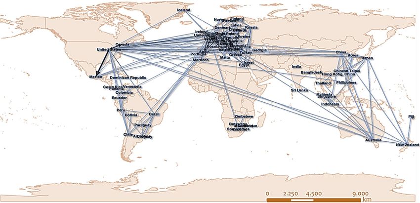
www.nature.com/scientificreports/
scientific research is multidisciplinary, broad, and c omplex2,5,7,21–23, illustrating the linkage of COVID-19 with all
aspects of everyday life, along with the intention of the humanity to get ahead in the fight against the pandemic.
Although a thorough review of the vast and multidisciplinary COVID-19 literature is an ongoing and future
challenge for epistemology researchers, the relationship between the pandemic’s spreading and the intercon-
nected socioeconomic structure of the modern world is more than evident in the literature2,12,16,24–27. At the
microscopic level, the relationship between individual connectivity and COVID-19 spread (transmission) builds
on clinical and epidemiologic terms. This approach has already enjoyed fruitful research contributing to the
understanding and pandemic m anagement28–30. In macroscopic terms, the effect of interconnectedness on the
pandemic’s spread is mainly studied on a dual basis, either within or between countries (in a cross-country
framework). The first approach covers all topics of interest about the pandemic, such as regional outbreaks and
spread due to imported cases31,32, mobility, and travel restrictions14,15, the effects of lockdown17,33, and others4,34.
Even when is implemented on an international scale, the within-countries approach conceives interconnected-
ness as an intrinsic property of countries, interpreting the uneven spread of the pandemic based on comparing
such intrinsic properties between countries. In addition, the second (cross-country) approach conceptualizes
the spread-channels (links) of the pandemic between countries by configuring variables or indicators approxi-
mating aspects of interconnectedness, such as the number of tourists, geographical distance, exports per capita,
motorway density, etc.35–37.
However, interconnectedness becomes better conceivable in the context of communication theory38,39, accord-
ing to which the infection of COVID-19 is the result of virus transmission between two i ndividuals3,40, namely
an elementary communication structure called either link or e dge41. Building on such pair-wise configuration,
the complex COVID-19 virus transmission system can excellently represent a network structure and be mod-
eled as a graph, as conceived by network science41–44, at any spatial and functional level. In the literature, this
cognition appears to become deeper. For instance, the authors o f45 applied social network analysis to track the
spread of COVID-19 in India and found that international travels were determinative of the pandemic outbreak
in the country. On the same basis, the work of46 studied a social network of the COVID‑19 spread in South
Korea, finding that the topology of the infection network was dependent on the policy measures applied by the
government to control the pandemic. The paper of47 constructed a multilayer network of social connectivity to
study the COVID-19 epidemic spread in Brazil and the country’s potential to manage the effect of the pandemic,
proposing the increase of social isolation (up to a lockdown) as the best option to preserve the functionality of
the healthcare system capacity. The work of48 developed a multilayer network methodology of the relationship
between socio-cultural and economic characteristics to identify the pandemic spreaders, resulting in a classifica-
tion of the countries according to their socioeconomic, population, Gross Domestic Product (GDP), health, and
air connectivity attributes. The authors of49 developed a network model of social contacts between individuals,
calibrating their model on data about COVID-19 spread in Wuhan (China), Toronto (Canada), and the Italian
Republic, using a Markov Chain Monte Carlo (MCMC) optimization algorithm. The results showed a good fitting
of the network model to empirical data and provided a tool for the health authorities to plan control measures
against the pandemic. The paper of13 used social network analysis to identify the clusters of the COVID-19
global spread and observed that the pandemic spread followed a route from China to West Asia, Europe, North
America, and South America according to three classifications. The authors o f50 developed a SAIR (Susceptible-
Asymptomatic-Infected-Removed) model on social networks to study the spread of COVID-19 and examined
the effectiveness of policy measures aiming to control the pandemic. Also, the authors of51 used agent-based
simulations based on the SEIR (susceptible–exposed–infectious–recovered) model to show that two network
intervention strategies dividing or balancing social groups can substantially reduce transmission while sustaining
economic activities. On a similar framework, the authors o f52 developed a contact network to study the city-
level transmission using an infectious agent spread (SEIR) model, showing that precise knowledge of epidemic
transmission parameters is not required to build an informative model of the spread of disease.
f53 studied the impact of human mobility networks on the COVID-19 onset in 203 different
Further, the work o
countries. The authors used exponential random graph models to perform an analysis of the country-to-country
global spread of COVID-19. The analysis showed that migration and tourism inflows were factors increasing
the probability of COVID-19 case importations. The authors of54 studied a knowledge network model of semi-
supervised statistical learning constructed on aerial mobility data of Hong Kong and Wuhan. The purpose of
the study was to determine the early identification of infectious disease spread via air travel and align the need
to keep the economy working with open connections and the different dynamics of national pandemic curves.
The work of55 applied a network inference approach with sliding time windows to capture the spatiotemporal
influence of infections and trace the spread of the pandemic in New York and the USA. The paper o f56 employed
an agent-based model to nearly 1.6 million firms in Japan and simulated the pandemic’s propagation, where they
evaluated lockdown scenarios of Tokyo, Japan. On a similar conceptualization, the authors o f57 examined how
the economic effects of lockdowns in different regions interact through the supply network of 1.6 million firms
in Japan. The analysis showed that a region’s upstream-ness, the intensity of loops, and supplier substitutability
in supply chains with other regions largely determine the economic effect of the region’s lockdown. The paper
of58 investigated the impact of COVID-19 on global air transportation at different geographical scales, namely
worldwide, international country, and domestic airport networks, for representative cases, and found that the
impacts of the pandemic were concordant, in intensity, with the geographical scale. The work o f59 developed a
complex network of COVID-19 correlations between 122 countries and empirically investigated the network
connectedness influencing macroeconomic and social factors. The analysis showed that population density,
economic size, trade, government spending, and quality of medical treatment are significant macroeconomic
factors affecting COVID-19 connectedness in different countries.
As is evident from the previous review, the network paradigm provides an insightful approach for study-
ing and understanding the spreading of the pandemic within the context of the modern world’s connectivity.
Scientific Reports | (2022) 12:666 | https://doi.org/10.1038/s41598-021-04717-3 2
Vol:.(1234567890)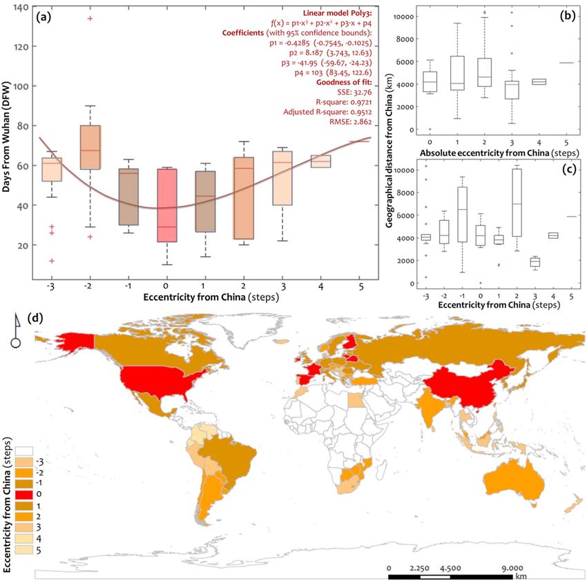
www.nature.com/scientificreports/
This approach goes beyond other non-network counterparts, which conceive interconnectedness either as an
intrinsic property of countries4,27,33 or in terms of variables or indicators approximating aspects of cross-country
interaction35–37. Therefore, using the network paradigm allows developing graph models representing intercon-
nected structures at various geographical scales. However, there is still a long way to go on the network analysis
of the interconnectedness of COVID-19 because current empirical approaches are relatively restricted compared
to the broad range of human economic activity. In particular, the relevant research mainly applies to (a) social
network models45–51, (b) supply and logistic n etworks56,57, and (c) networks of human m obility53,54,60. Moreo-
ver, due to big-data demand, relevant studies implemented at the global scale are considerably fewer. Toward
responding to this demand, this paper focuses on the patterns and causes (first strand) of the COVID-19 spread.
It develops a multidimensional methodological framework for understanding the spatio-temporal spread of
the pandemic in the context of the global economy modeled as an interconnected cross-country structure.
Therefore, this study goes beyond the previous complex network approaches by constructing a global network
model incorporating dimensions of topology, geography, and economic openness. To do so, it conceptualizes
worldwide interconnectedness based on economic g lobalization61 and, specifically, by constructing a network
model of international tourism flows.
In terms of transport geography62 and spatial economics63, a tourism network belongs to the family of trans-
portation networks. However, it is quite different from a typical transportation network, such as road, railway,
maritime, or air transport n etwork43,64–66, both in terms of structure and functionality. First, a tourism network
has a specific economic configuration of its transport demand64,67,68, which involves movements for tourism pur-
poses outside the country of residence. On the contrary, in a typical transportation network, the economic forces
driving the transport demand are broad and unspecified since they may refer to trade, occupation, recreation,
health, education, etc.62,69. Therefore, as far as the economic configuration of transport demand is concerned, a
tourism network is well-defined within a unified functional framework (or economic activity), while a typical
transport network (except a multilayer model) is not and is multivariable. However, in terms of modal configu-
ration, a tourism network is multimodal because movements may occur through all transportation modes62. In
contrast, a typical transport network usually is defined within a single transportation mode43. Finally, in terms
of network topology43, a tourism network is more topological than geometric64,67,68, as a typical transportation
network usually is. In particular, in a tourism network, edges are usually defined as accessibility links and not
as routes or transportation c hannels62,67. Within this context, the network model of international tourism flows
constructed in this paper suggests a good p roxy35,45,53 for the outbreak of the pandemic because (a) it provides
a comprehensive economic setting (tourism), (b) is integrated in terms of modal configuration, and (c) is more
representative in terms of network accessibility.
This study builds on a three-dimensional conceptual model to analyze the worldwide spatio-temporal spread
of COVID-19. It incorporates one dimension approximating the interconnectedness of the international tourist
mobility, a second one describing the openness of countries to the globalized economy, and a third one expressing
the spatial impedance to transportation. By constructing a single network model, this paper proposes an inte-
grated framework for the study of the spatio-temporal spread of COVID-19. It also contributes to the literature
with more realistic models of the worldwide interconnected system, where COVID-19 and other pandemics are
spreading. The remainder of this paper is structured as follows: second section presents the methodological and
conceptual framework of the study, third section shows the results of the analysis and discusses them within the
context of regional and geographical sciences, and finally, in last section, conclusions are given.
Methods
Conceptual framework. This paper develops a multidimensional (3D) model for understanding the une-
ven (cross-country) spread of COVID-19 in the context of the globally interconnected economy. The conceptual
framework of the study is illustrated in Fig. 1 and consists of five steps. In the first step, we configure the vari-
able expressing the temporal spread of the pandemic, measured in terms of the time at which the first infection
emerged from Wuhan to each country (DFW). This variable provides a good proxy for interconnectedness
because it quantifies the impedance of the pandemic flows between countries, namely the level at which each
international link resists or facilitates the transmission of the pandemic flows in the network. In the second step,
we construct a graph model of the Global Tourism Network (GTN), on which we compute fundamental (node)
network measures. In the third step, the study develops a three-dimensional (3D) conceptual model to analyze
the worldwide spatio-temporal spread of COVID-19. This 3D model includes different variables grouped by
its dimensions. The first dimension (component) approximates the interconnectedness of international human
mobility (1D: global network interconnectedness). The second one describes the spatial impedance to transpor-
tation (2D: spatial impedance).
The third dimension expresses the economic openness and attributes of countries in the structure of the
globalized economy (3D: economic structure and openness). Variables belonging to the first dimension are con-
figured from the available network measures of the GTN, whereas the other predictors extract from secondary
databases. In the fourth step, the analysis applies toward different combinations (approaches) of the available
dimensions. The first combination (DFW, 1D) expresses the embedding of variable DFW to the GTN’s space, as
described by the spatial distribution of DFW in the GTN’s map. The second approach (DFW, 1D, 2D) is a net-
work analysis incorporating structural and geographical information of the GTN. Finally, the third approach is
an empirical analysis including all available information of the 3D model. In the final (fifth) step, we discuss the
results and formulate conclusions. Overall, this 3D conceptual model examines if patterns in the cross-country
temporal spread of COVID-19 relate to various aspects of interconnectedness in the structure of the worldwide
mobility system. Within this context, it provides insights into the topological, geographical, and socioeconomic
factors affecting the uneven spread of the pandemic.
Scientific Reports | (2022) 12:666 | https://doi.org/10.1038/s41598-021-04717-3 3
Vol.:(0123456789)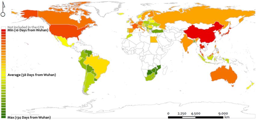
www.nature.com/scientificreports/
Figure 1. The conceptual framework of the study.
Figure 2. The graph model of the directed GTN (data of the year 2018, own elaboration based on ESRI ArcGIS
10.50; https://www.arcgis.com).
Graph modeling and analysis. This study uses the network paradigm, as conceived by network
s cience42–44, to represent the Global Tourism Network (GTN) into a graph. Generally, a graph model is a pair-set
of nodes and edges41, quantitatively modeled using connectivity and weight matrices. In comparison with other
models of socioeconomic or spatial interaction, graphs have the advantage of including, in a single model, both
structural and functional information70, available both on a local (node, neighborhood) and global (the total
network) scale. This property makes graph models more effective in describing real-world s ystems71 because it
equips them with a double (hybrid) microeconomic and macroeconomic setting. The Global Tourism Network
(GTN) is constructed on data of the year 2018, extracted from the Organization for Economic Co-operation and
Development72. The available data include records of the top-5 markets (including either OECD or non-OECD
countries) of the inbound and outbound tourism flows per OECD country. The GTN (Fig. 2) is a directed
and weighted graph G(V,E), where nodes (i) correspond to tourism-destination countries, and links (ij) to the
annual number of tourists originating from a node (country of origin) i ∈ V and visited node j ∈ V (destination
Scientific Reports | (2022) 12:666 | https://doi.org/10.1038/s41598-021-04717-3 4
Vol:.(1234567890)
www.nature.com/scientificreports/
Measure (symbol) Description Math formula References
Nomenclature
A pair set consisting of a node-set V and an edge-set E
Graph G(V,E) 41,43
In graph G(V,E), n expresses the number of nodes and m the number of links
Network measures
ki = m(i) = mi = δij = δij ,
The number of graph edges being adjacent to a given node i j∈V (G) j∈V (G)
41
Node degree (k)
It expresses the communication potential of a node
1, if eij ∈ E(G)
where δij =
0, otherwise
ki − = mi − = δij −, where
The number of incoming edges being adjacent to given node i (applicable in directed j∈V (G)
41,43
In-degree (k–)
graphs)
1, if eij ∈ E(G)
δij =
0, otherwise
ki − = mi − = δji −, where
The number of outgoing edges being adjacent to given node i (applicable in directed j∈V (G)
41
Out-degree (k +)
graphs)
1, if eji ∈ E(G)
δij =
0, otherwise
The sum of weights (wij) of the links (eij) being adjacent to a given node i si = s(i) = δij · dij ,
Node strength (s) The δij operator is the Kronecker delta function yielding one for links belonging to j∈V (G) 41,43
graph G where dij = w(eij ) in km
n
1
Average degree k
The mean value of node degrees ki, where i represents a network node 74
�k� = n · ki
i=1
The probability a node i to have E(i) neighbors connected
Local clustering coefficient (C(i)) Computed on the number of triangles configured by node i to the number of the total C(i) = E(i)
ki ·(ki −1)
41
triplets ki(ki–1) shaped by this node
A proportion is defined by σ(i) shortest-paths that pass through node i to the total
Betweenness centrality (CB) shortest-paths σ in the network 75
CB(i) = σ (i) σ
It measures the intermediacy of network paths
Computed on the average path-lengths d(i,j) originating from a given node i ∈ V to all 1
n
Closeness centrality (CC) other nodes j ∈ V in the network CC(i) = n−1 · dij = d̄i 75
It is a measure of accessibility j=1,i� =j
Eccentricity (e(u)) The longest path p(u,j) in the network from a given node u ∈ V 75
e(u) = max p(u, j)
j ∈ V
Table 1. Measures of network topology used in the analysis of GTN.
country). The GTN is also a connected graph, composed of n = 75 nodes and m = 179 links (edges) and modeled
in the L-space representation43, where nodes are connected if they are successive stops on a given route. Intui-
tively, the L-space (also called space of stations) resembles a physical representation because it illustrates direct
connections between geo-referenced nodes but differs in the way that edges are shown, drawn as linear segments
instead of real-shaped curves. This difference reduces modeling complexity, which is less costly than the physi-
cal representation because it requires just a pair of elements to display a connection (source node, target node).
In general, the L-space representation is more geometric than others that are more topological (see43,65) and
therefore is preferable for cases where the systems’ geometry matters. Within this context, the GTN is modeled
in the L-space representation, where nodes are geo-referenced at the coordinates of the countries’ capital cities
by using the Web Mercator projection73.
After constructing the graph model of the GTN, we compute fundamental network measures, as shown in
Table 1. These measures are extracted from the relevant literature41,43,74,75 and capture different aspects of the
GTN’s topology, such as connectivity, intermediacy, clustering, and accessibility.
The 3D model configuration. To study the international spread of COVID-19, we construct and col-
lect twenty-four (24) variables, shown in Table 2. The first one includes epidemiologic information referring to
the time-distance (measured in days from Wuhan—dfW) of the first confirmed case (infection) per country,
whereas the other 23 variables group into the categories of the overall 3D conceptual approach. For the configu-
ration of the variables included in the 1 st category (global network interconnectedness), the analysis employs
graph modeling to represent the globally interconnected system of tourism mobility as a complex network. The
variables included in the other two categories (2D: spatial impedance, and 3D: economic openness) originate
from various Web sources of secondary data72,73,76–83, where cases only referring to the countries included in the
GTN are included in the variables’ configuration. Within this context, all the available variables of Table 2 have
length 75, with each element referring to a GTN node (country).
Quantitative tools and methods. This paper builds on a multidimensional network analysis employing
methods of statistical mechanics, such as descriptive and statistical-inference analysis, parametric fitting, and
non-parametric estimation methods84–88, to study the uneven spread of the COVID-19 pandemic. The descrip-
tive methods used in the analysis are graphic methods aiming to display different aspects of distributions of
Scientific Reports | (2022) 12:666 | https://doi.org/10.1038/s41598-021-04717-3 5
Vol.:(0123456789)www.nature.com/scientificreports/
Group Symbol Description Source/references
COVID-19 emergence time: The time where the first COVID-19 infection emergence in a
EPIDEMICS DFW 82
country. Is measured in days from Wuhan (dfW)
DEG Node degree: The number of connections per GTN node (country)
IN.DEG Node in-degree: The number of incoming connections per GTN node
OUT.DEG Node out-degree: The number of outgoing connections per GTN node
41
Node strength: The sum of weights (tourists) of the (incoming and outgoing) connections per *
STR
GTN node
IN.STR Node in-strength: The sum of weights (tourists) of the incoming connections per GTN node
OUT.STR Node out-strength: The sum of weights (tourists) of the outgoing connections per GTN node
1D global network interconnectedness
C Node clustering coefficient: The clustering coefficient per GTN node
CB Node betweenness centrality: The betweenness centrality per GTN node
CC Node closeness centrality: The closeness centrality per GTN node
75
ECC Node eccentricity: The eccentricity per GTN node *
Eccentricity from China: The eccentricity of a GTN node whether China is considered as
the GTN’s center. Is defined by the relation ECCFC(i) = ECC(i)–3, yielding integer outcomes
ECCFC
(where negative values imply that these cases are more central in reality than China in the
GTN topology)
Coastal indicator: Dummy (binary indicator) variable indicating whether a country is coastal
CST
(1) or not (0)
Own elaboration, based on73
Distance from China: The shortest geographical distance of a country from China (measured
DSTFC
in km)
2D spatial impedance RDL Road length: The length of the road network in each country (measured in km) 76
RLL Rail length: The length of the rail network in each country (measured in km) 80
PRT Ports: The number of active ports in each country, for the year 2020 83
APRT Airports: The number of active airports in each country, for the year 2020 79
Overall KOF Globalisation Index: Composite index measuring economic, social, and political
GI 77
globalization (yearly; from 1970 to 2017). Data refer to the year 2017
Gross Domestic Product (GDP): GDP is the sum of gross value added by all resident produc-
ers in the economy plus any product taxes and minus any subsidies not included in the value
GDP of the products. It is calculated for the year 2017, without making deductions for depreciation 81
of fabricated assets or depletion and degradation of natural resources. Data are in constant
2010 U.S. dollars
Total factor productivity (TFP): Composite indicator expressing (loosely) the growth
TFP achieved due to labor and capital productivity factors. It is computed on constant national
3D economic structure and openness prices (2011 = 1)
78
Population: The number of citizens of the country according to the most recent national
POP
census
Human Capital: Human capital index based on (a) years of schooling and (b) returns on
HC
education
GDP per capita: The GDP divided by mid-year population. Data are in constant 2010 U.S.
GDP.pc 81
dollars
TFP.pc Total factor productivity per capita: The TFP, divided by the country’s population 78
Table 2. Variables participating in the analysis of COVID-19 global spatio-temporal spread. *Own elaboration
for the GTN, based on72 database for the year 2018.
the available data, either in a spatial context (spatial distribution maps, see89) or in a single-variable (boxplots
plotting the median, Q1 and Q3 quartiles, and potential outliers and extreme values) or pair-wise (boxplots and
scatter-plots plotting ordered pairs of numeric values corresponding to different variables) consideration86,90.
In terms of statistical inference, the analysis builds on the formulation of error bars representing confidence
intervals (CIs) constructed for estimating (at a 95% confidence level) the difference of the mean values between
groups of cases within a variable86. These error bars graphically illustrate an independent samples t-test of the
mean90. When they intersect with the zero-line (horizontal axis), the mean values of the groups cannot be con-
sidered statistically different, whereas when they do not intersect they can.
Parametric fitting techniques are applied to estimate the parametric curve that best describes the variability
of the dataset displayed in a scatter plot. The available fitting curves examined in this part of the analysis are
linear (1st-order polynomial, abbreviated Poly1), quadratic (2nd-order polynomial, Poly2), cubic (3rd-order
polynomial, Poly3), one-term power-law (Power1), one-term Gaussian (Gauss1), one-term exponential (Exp1),
and one-term logarithmic (Log1). All available types of fitting-curves can generally be described by the general
multivariate linear regression m odel86:
b i
ŷ = b1 f1 (x) + b2 f2 (x) + . . . + bn fn (x) + c = fi (x) + c, (1)
Scientific Reports | (2022) 12:666 | https://doi.org/10.1038/s41598-021-04717-3 6
Vol:.(1234567890)www.nature.com/scientificreports/
Figure 3. Heat map illustrating the spatial distribution of the temporal spread variable (DFW) expressing the
number of days from Wuhan (dfW) since the first case emerged in a country (the days of the first infection per
country), for the countries included in the GTN (own elaboration based on ESRI ArcGIS 10.50; https://www.
arcgis.com).
where f(x) is either logarithmic f(x) = (log(x))m, or polynomial f(x) = xm, or exponential f(x) = (exp{x})m, with
m = 1, 2, 3, or power f(x) = ax. The curve-fitting process estimates the bi and a (where is applicable) parameters that
best fit the observed data and simultaneously minimize the square differences yi − ŷi86, as is shown in the relation:
n
n
2
2
bi
(2)
min e = yi − ŷi = min yi − fi (x) + c
i=1 i=1
The parameter estimation uses the Least-Squares Linear Regression (LSLR) method, based on the normality
assumption for the differences e N(0, σe2 )86,90.
Finally, the non-parametric kernel density estimation (KDE) method estimates the probability density func-
tion of a random variable. The KDE method returns an estimate fˆ (x) of the probability density function for the
sample data in a vector variable x. This estimate is based on a normal kernel f unction84,85 and is evaluated at
equally-spaced (100 in number) xi points covering the data’s range. In particular, for a uni-variate, independent,
and identically distributed sample x = (x1, x2, …, xn), extracted from a distribution with unknown density (at
any given point x), the kernel density estimator fˆh (x) describes the shape of the probability-density function ƒ,
according to the r elation84,85:
n n
1 1 x − xi
fˆh (x) = Kh (x − xi ) = K , (3)
n nh h
i=1 i=1
where K is the kernel (a non-negative) function and h > 0 is a smoothing parameter called bandwidth, which
provides a scale (desirably the lowest possible h) in the kernel function Kh(x) = 1/h·K(x/h) depending on the
ilemma91.
bias-variance trade-off d
Overall, the multilevel analysis builds on statistical mechanics of the available network, socioeconomic, and
geographical variables to conceptualize the worldwide uneven spatio-temporal spread of COVID-19 within the
context of the global interconnected economy represented by the GTN.
Results
Descriptive (1D) analysis. At the first step of the analysis, we construct the heat map of Fig. 3, which
shows the worldwide spatial distribution of the COVID-19 emergence per country (variable DFW expresses
the number of days from Wuhan since the first infection). This heat map shows some clusters in the world
map with distinguishable geographical patterns. The first cluster includes the red-colored countries, expressing
cases where the first COVID-19 infection emerged relatively soon after the pandemic started in Wuhan (clus-
ter of shortly infected countries). This cluster mainly includes countries neighboring China, along with North
America, Australia, and Western Europe. The geographical distribution of this cluster configures a spatial pat-
tern shaping an arc consisting of North America–Western Europe–Russian Federation–China–India–Thailand
Islands–Australia, and covers the northern and eastern part of the world map.
Scientific Reports | (2022) 12:666 | https://doi.org/10.1038/s41598-021-04717-3 7
Vol.:(0123456789)www.nature.com/scientificreports/
The second cluster (Fig. 3) includes the green-colored countries, where the first COVID-19 infection emerged
relatively far from the day the pandemic began in Wuhan. This cluster (of late infected countries) mainly distrib-
utes along the meridian zone, including (a) South America, Southern Africa, and Indonesia, (b) a sub-cluster
of countries in Central Europe and the Western Mediterranean basin, and (c) Turkey. Finally, the third cluster
includes the yellow-colored cases, which describe countries of average emergence of the pandemic from Wuhan
(~ 58 days). This cluster configures a scattered spatial pattern including European and American countries,
distributed along a southwest (in Latin America) and north (in Europe) line.
Overall, this descriptive analysis provides visual evidence about the global dynamics of the pandemic’s spread
in the context of the GTN. As can be observed, proximity is evident in the distribution patterns of the COVID-19
spread. This observation complies with relevant findings36,37,58 about (a) the importance of geographical distance
in the spread of the pandemic, and (b) the empirical knowledge stating that neighborhood connections undertake
the highest traffic in spatial and transportation networks43,62. However, this is not the whole picture describing
the spatial patterns in Fig. 3, which in such a case would follow just a circular distribution of color intensity. The
clustered and asymmetric spatial distribution previously described in the heat map implies the effect of more
forces than just proximity in the configuration of the COVID-19 spread, bringing into the light those theories
about the socioeconomic factors determining transportation flows due to the differential demand (or attractive-
ness) emerging in space62. Therefore, this (1D) approach contributes to shaping an initial picture and motivates
applying further research going deeper in the study of COVID-19 spatial spread.
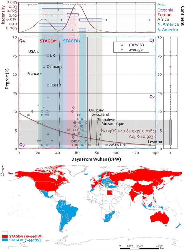
Network (2D) analysis. In the second part of the analysis, we construct a multilayer diagram including
scatterplot, boxplots, and ks-density components (Fig. 4), to study the distribution of the pandemic’s emer-
gence per country relative to the GTN network interconnectedness. The main window of the scatterplot (DFW,
DEG≡k) shows the correlation between the days since the first infection from Wuhan (dfW) and the node-degree
(k) of the GTN countries. At the axes, the boxplots illustrate the main aspects of the distributions (median, Q1
and Q3 quartiles, potential outliers, and extreme values) of the corresponding variables (DFW and k), where they
further divide into continent groups in the horizontal axis (measuring days from Wuhan). In Fig. 4, according
to the ks-density plot and the pattern of the scatterplot shown in the main window, we can observe two stages
in the COVID-19 temporal spread throughout the GTN. These stages configure distinguished bell-shaped areas
shown in the ks-density curve, defined by the cutting point of the 44th day from Wuhan (t = 44 dfW). The detec-
tion of these stages is due to the network configuration that applied a filter to the world countries keeping only
those 75 belonging to the GTN. In particular, the first stage includes nodes infected before the 44th day from
Wuhan (≤ 44 dfW), mainly described by the outbreak in Asia and North America (as is evident by the country
boxplots). The second one includes nodes infected after the 44th day from Wuhan (> 44 dfW), described by the
outbreak in Europe, South America, and Africa. The outbreak in Oceania spreads along both stages but is slightly
positively asymmetric, having its median value placed at the first stage. This outcome complements and revises
with broader information the finding of the authors of13, who observed three clusters in the COVID-19 global
spread, following a route from China to West Asia, Europe, North America, and South America. Although the
pandemic emerged in Europe mainly in the second stage, the cases of the UK (k = 25), Germany (k = 22), France
(k = 20), and the Russian Federation (k = 17) faced COVID-19 in the first stage. All these European countries are
GTN hubs (nodes of high degree) and belong to the Q4 quartile (t ≤ 44 dfW, ki > 15), as is shown in Fig. 4.
On the other hand, the late infected nodes mainly concern African countries belonging to the Q2 quartile
(t > 44 dfW, ki ≤ 15) and, in terms of the GTN connectivity, they are spokes, namely nodes of one connection, with
degree k = 1. According to the ks-density distribution, most nodes (> 85%) faced the pandemic between the 20th
and the 70th dfW. The interquartile range (50% of data) at the period is 30–64th dfW. A parametric fitting curve
applies to the average degree (< k >) data to shape a picture of how average connectivity behaves as a function of
the COVID-19 emergence time (t = DFW) in the GTN. The (adjusted) coefficient of determination (R2 = 0.924)
shows a high correlation < k > = f(t) between these two variables, described by a decaying exponential pattern
with mathematical expression < k > = f(t) = 10.82·exp(− 0.018t). This exponential decay pattern implies that, on
average, the GTN hubs are early infected by the pandemic (which is also verified by the fact they belong to the
first stage), while lower degree nodes were late infected. In general, this fitting curve, along with the multilayer
scatterplot, shows that the relationship between interconnectedness in the GTN and the COVID-19 emergence
is not likely to be a result of randomness, implying that network interconnectedness is related to the temporal
spread of the pandemic within a causative context. This finding provides a context quantitatively defining the
relationship between global interconnectedness and COVID-19 spread. This context can support relevant studies
observing that international connectivity is determinative to the pandemic’s o utbreak45,48.
In geographical terms, the map in Fig. 4 illustrates the spatial distribution of the two stages of COVID-19’s
temporal spread in the GTN. As can be observed, the first stage of the pandemic’s temporal spread mainly covers
the northern hemisphere, whereas the second stage covers the southern hemisphere, with notable exceptions the
cases of Central Europe and Australia, respectively. As is evident from the previous analysis, the spatial patterns
of the two-stage worldwide temporal spread of COVID-19 in the GTN appear as more a matter of network inter-
connectivity (node degree) than of spatial proximity. This observation complements these works focusing either
on the importance of geographical d istance36,55,58 or on the importance of international c onnectivity45,48,53 in the
spread of the pandemic, and develops a common context for the study of the pandemic’s outbreak. The boxplots
of Fig. 5 are constructed to study in more detail the effect of proximity in the temporal spread of the pandemic
throughout the GTN structure. The boxplots illustrate how the variables of COVID-19 emergence time (Fig. 5a),
measured in days since the first infection from Wuhan, and spatial (geographical) distance (Fig. 5b,c) distribute
along groups configured by the node-eccentricity of the GTN. To provide a reference to the case of China, due
to its importance in the spread of the pandemic, we center the node-eccentricity to China by subtracting all
Scientific Reports | (2022) 12:666 | https://doi.org/10.1038/s41598-021-04717-3 8
Vol:.(1234567890)www.nature.com/scientificreports/
Figure 4. Multilayer scatterplot (DFW,k) showing the correlation between the days since the first infection
from Wuhan (DFW) and the node-degree (k) of the GTN. Boxplots in each axis illustrate the distribution of
each variable, where DFW further separates into continent groups. Shaded zones within the scatterplot express
interquartile ranges of each boxplot. Quadrants Q1, Q2, Q3, and Q4 in the scatterplot area correspond to median
lines. The fitting curve f(x) is applied to average degree values (< k >), expressed by cross “+” symbols. At the
bottom, the map shows the spatial distribution of the two stages defined by the ks-density curve (maps are own
elaboration based on ESRI ArcGIS 10.50; https://www.arcgis.com).
Scientific Reports | (2022) 12:666 | https://doi.org/10.1038/s41598-021-04717-3 9
Vol.:(0123456789)www.nature.com/scientificreports/
Figure 5. Boxplots expressing (a) the days since the first infection from Wuhan (DFW) for each class of the
GTN’s eccentricity centered at China (abbreviated: eccentricity from China), the eccentricity of which is 3 steps
(also shows the fitting curve of best determination applied to average values), and the geographical distance
from Wuhan (DFW) for each class of (b) absolute and (c) non-absolute eccentricity from China. Also, the
diagram shows the fitting curve of best determination applied to the average values. The bottom map (d) shows
the spatial distribution of the eccentricity from China (maps are own elaboration based on ESRI ArcGIS 10.50;
https://www.arcgis.com).
scores by China’s eccentricity, which equals 3 steps. Therefore, we compute a new variable named “eccentricity
from China” (ECCFC), defined by the algebraic difference ECCFC(i) = ECC(i)–3 according to Table 2, where i is
a GTN node. Although ECCFC measures distance, its algebraic definition also allows receiving negative integer
values, implying that these cases are more central in reality than China in the GTN topology. For the sake of
completeness, we also consider in the analysis the absolute of the ECCFC variable.
In descriptive terms, the boxplots of Fig. 5 illustrate the correlations of the pairs of variables (DFW, ECCFC),
(DSTFC, ECCFC), and (abs(DSTFC), ECCFC). As is evident in Fig. 5a, the curve fitting applied to the boxplot
medians of the eccentricity groups shapes a cubic pattern, which describes the median-data variability under a
high level of determination (adj.R2 = 0.9512). This “U”-shaped pattern yields a global minimum at the value of
ECCFC(i) = 0, which implies that, on average, the countries where the pandemic first emerged are those with the
same node-eccentricity as China, in the GTN. In all the other cases (nodes), the values of COVID-19 emergence
Scientific Reports | (2022) 12:666 | https://doi.org/10.1038/s41598-021-04717-3 10
Vol:.(1234567890)www.nature.com/scientificreports/
Figure 6. Error bars of 95% confidence intervals (CIs) for the average differences diff(xi )
, computed on
standardized variables (ranging from 0 to 1) between the groups of cases x(t < 44DFW) and x(t ≥ 44DFW)
defined by the cutting value t = 44DFW (the number of days since the first infection in Wuhan), for each of the
available network and economic variables (x1, x2, …, x19). Labels shown in bold font have significant differences.
time shape and almost symmetric distribution along both sides of the group of China’s eccentricity. Although
this pattern regards averages (and more accurately, to the extent that the median-values are representative of the
cases included in a boxplot), this observation implies that the center of the spread of the pandemic in the GTN
was not only China, but the core of countries having the same score of eccentricity as China. In other words,
it implies that the center of the pandemic spread includes all these nodes (countries) that are as central in this
network as China is.
As can be observed in the map of Fig. 5d, these countries, belonging to the eccentricity-core of China, are
not described by geographical proximity with China, but they are as central as China in the GTN. This finding is
hina2,23,27,36,61 in the spread of the pandemic
striking because it proposes reconsidering the certain central role of C
within the context of network connectivity. In particular, this result suggests that China has played a critical
role in the virus spread not because of the country’s first outbreak of COVID-19 worldwide, but because of the
country’s importance to the network connectivity, as a hub. This observation is further supported by the results
of Fig. 5b,c , showing that spatial proximity does not seem to be particularly related to the temporal spread of the
pandemic (DFW) because curve-fitting does not yield any pattern with considerable determination (R2 > 0.5).
Intuitively, the median-values arrangement in the boxplots in Fig. 5b,c approximates an almost linear pattern
in parallel to the horizontal axis, which might imply that the temporal spread of COVID-19 is indifferent to
geographical proximity. In this part, the overall approach highlights the importance of network centrality and
thus the critical role of hubs (as China is) in the worldwide temporal spread of the pandemic (to the extent that
centrality is described by the metric of eccentricity, measuring central positioning in the network).
Empirical (3D) analysis. In the final step of the analysis, we examine which variables included in the
3D-conceptual model of Table 2 can be considered significant determinants for the worldwide spatio-temporal
spread of COVID-19, in the GTN. To do so, we apply a series of t-tests to compare the means between the groups
defined by the two stages of the temporal spread of the pandemic. For better supervision of the results, the error
bars shown in Fig. 6 visualize the t-tests, where each variable is standardized to the interval [0,1] so that the
results of the t-tests are comparable. When the error-bars intersect with the horizontal axis (zero-line), the group
mean values can be considered statistically equal, under a 95% certainty. When error bars do not intersect the
zero-line, they can be considered statistically different (one group performs better than the other).
As can be observed in Fig. 6, in terms of network interconnectedness (1D conceptual component), the GTN
nodes (countries) belonging to the first stage of temporal spread are cases with a higher (a) degree (variable DEG),
expressing the number of connections of a node in the GTN; (b) outgoing degree (variable OUT.DEG), express-
ing the number of outgoing connections of a node in the GTN; (c) absolute eccentricity from China (variable
EECFC(ABS)), expressing the network binary distance from China; (d) strength (variable STR), expressing the
sum of incoming and outgoing tourists a GTN-node annually mobilizes, (e) incoming strength (variable IN.
STR), expressing the sum of incoming tourists a GTN-node annually receives; and (f) outgoing strength (vari-
able OUT.STR), expressing the sum of outgoing tourists a GTN-node annually sends to other destinations. The
Scientific Reports | (2022) 12:666 | https://doi.org/10.1038/s41598-021-04717-3 11
Vol.:(0123456789)www.nature.com/scientificreports/
t-tests applied to the variables of this conceptual component indicate that network interconnectivity and central
structure are significant determinants in the early global temporal spread of COVID-19.
In terms of spatial impedance (2D conceptual component), the GTN countries belonging to the first stage of
temporal spread are cases (a) with more coastal geomorphology (variable CST), (b) they have larger road (variable
RDL) and rail lengths (variable RLL), and (c) a greater number of ports (variable PRT) than those included in
the second stage of temporal spread. An interesting “insignificant” result in this conceptual group is the variable
APRT describing the number of airports included in the GTN countries. At a glance, this observation opposes
ndings45,53,54,58 stating that air travel and connectivity are major determinants of the pandemic’s
the literature fi
spread. However, in conjunction with the significant t-tests observed for the degree (DEG) and strength (STR)
variables (included in the network interconnectedness group), the insignificant performance of the APRT vari-
able implies that the airport network becomes a significant determinant in terms of connectivity rather than of
infrastructure capacity. Regardless of the participation of the APRT variable, the t-tests applied to the variables
of the 3d conceptual component illustrate how land and maritime transport capacity (which are critical aspects
of transport integration) significantly affected the early temporal spread of the pandemic worldwide.
Finally, in terms of economic openness (3D conceptual component), the GTN countries belonging to the
first stage of temporal spread have a higher (a) globalization index (variable GI), (b) GDP and GDP per capita
(variable GDP.pc), and (c) total factor productivity per capita (variable TFP.pc) than those included in the second
stage of the COVID-19 temporal spread in the GTN. These results come in line with those works observing
the importance of globalization on the spread of the pandemic2,58,61 and with others identifying productivity
as a major pandemic s preader2,48. Generally, the t-tests applied to the variables of this conceptual component
show that the countries with higher economic openness (those more integrated into the globalized economic
structure) were subjected earlier to the pandemic than those of lower economic openness. Overall, the t-test
analysis provides an integrated framework for understanding the uneven spread COVID-19, showing that net-
work interconnectedness, economic openness, and transport integration are key determinants in the early global
temporal spread of the pandemic.
Conclusions
This paper developed a multilevel methodological framework for understanding the uneven spatio-tempo-
ral spread of COVID-19 in the context of the globally interconnected economy. The framework is built on a
three-dimensional conceptual model, incorporating one dimension for approximating the interconnectedness
in worldwide human mobility, a second one for the global economic openness, and a third one for the spatial
impedance to transportation. The analysis applied to a major temporal variable expressing the pandemic’s emer-
gence (measured in days from Wuhan since the first infection) and to another twenty-three variables grouped
into three categories (dimensions) of a 3D conceptual model. Firstly, the descriptive (1D) analysis revealed three
clusters in the world map with distinguishable geographical patterns of the pandemic temporal spread. The first
one of early infected countries configured a geographical arc distributed throughout the countries neighboring
China, North America, Australia, and Western Europe. The second cluster of late-infected cases was distributed
mainly along the meridian zone of South America, Southern Africa, and Indonesia, including a sub-cluster
with countries of Central Europe, the Western Mediterranean basin, and Turkey. The third cluster configured a
scattered spatial pattern throughout the globe. The network (2D) analysis led to further specialization of these
findings and revealed two main stages in COVID-19’s temporal spread throughout the GTN. The first included
nodes infected by the pandemic before the 44th day from Wuhan (≤ 44 dfW) and described the outbreak in Asia
and North America. The second one included nodes infected after the 44th day from Wuhan (> 44 dfW) and
described the outbreak in Europe, South America, and Africa. Finally, the outbreak in Oceania spread along both
stages. In geographical terms, the first stage of the pandemic’s temporal spread appeared to be more a matter of
the northern hemisphere, whereas the second stage involved the southern hemisphere. Next, the analysis applied
to the average degree and temporal spread of the pandemic showed a decaying exponential pattern, indicating
that hubs in the GTN were early infected, while lower degree nodes were infected late by the pandemic. This pat-
tern showed that network interconnectedness is related to the temporal spread of COVID-19 within a causative
context. Further, the network analysis revealed a “U”-shaped pattern describing the correlation between network
eccentricity and the temporal spread of the pandemic, describing that the center of the pandemic’s temporal
spread in the GTN included China and the core of countries that are as central in the network as China is. This
finding is striking, implying that the importance of China in the spread of the pandemic is more a matter of its
hub connectivity in the GTN than the worldwide first emergence of the pandemic in the country. The analysis also
revealed that spatial proximity was not a major determinant of the temporal spread of the pandemic. Finally, the
empirical (3D) analysis applied to the total set of available variables indicated first that network interconnectiv-
ity and central structure are significant determinants of the early temporal spread of COVID-19, secondly that
countries with higher economic openness earlier submitted to the infection of the pandemic, and finally that land
and maritime transport integration significantly affected the early temporal spread of the pandemic worldwide.
Overall, this paper (a) revealed two major stages in the temporal spread of the pandemic within the context of
interconnected worldwide mobility networks, (b) highlighted the importance of network centrality in the world-
wide temporal spread of the pandemic, (c) showed that network interconnectedness, economic openness, and
transport integration are key determinants in the early global spread of the pandemic, and (d) revealed that the
spatio-temporal patterns of the worldwide spread of COVID-19 were more a matter of network interconnectivity
than of spatial proximity. These findings can provide useful insights not only for contributing to the scientific
knowledge but also for promoting current and future practices in epidemiology and public health management.
For instance, the mix and intensity of policy measures (personal protection; self and social isolation; local and
national lockdowns; etc.), aiming to support strategies against current or future waves of the (or a) pandemic,
Scientific Reports | (2022) 12:666 | https://doi.org/10.1038/s41598-021-04717-3 12
Vol:.(1234567890)www.nature.com/scientificreports/
can differentiate per country according to the tradeoff between the specific topological (connectivity), economic
(openness), and geographical (distance) attributes of the country in the spreading network. Provided that time
is extremely costly during the outbreak of a pandemic, countries with a more central topological position in a
virus spreading network should be more alerted and apply faster more severe measures than others, regardless
of the geographical distance of the country from the pandemic’s source. To do so, the success in the mix of such
measures depends on the profound knowledge about the position of a country in its network and economic
environment, toward which this paper contributes to a better understanding.
Received: 23 February 2021; Accepted: 30 December 2021
References
1. Anderson, R. M., Heesterbeek, H., Klinkenberg, D. & Hollingsworth, T. D. How will country-based mitigation measures influence
the course of the COVID-19 epidemic?. The Lancet 395(10228), 931–934 (2020).
2. Brodeur, A., Gray, D., Islam, A. & Bhuiyan, S. A literature review of the economics of COVID-19. J. Econ. Surveys 35(4), 1007–1044
(2021).
3. Demertzis, K., Tsiotas, D. & Magafas, L. Modeling and forecasting the COVID-19 temporal spread in Greece: An exploratory
approach based on complex network defined splines. Int. J. Environ. Res. Public Health 17, 1 (2020).
4. Ruktanonchai, N. W. et al. Assessing the impact of coordinated COVID-19 exit strategies across Europe. Science 369(6510),
1465–1470 (2020).
5. Gallo Marin, B. et al. Predictors of COVID-19 severity: A literature review. Rev. Med. Virol. 31(1), 1–10 (2021).
6. Oliveira, J. F. et al. Mathematical modeling of COVID-19 in 148 million individuals in Bahia. Brazil. Nat. Commun. 12(333), 1.
https://doi.org/10.1038/s41467-020-19798-3 (2021).
7. Yuce, M., Filiztekin, E. & Ozkaya, K. G. COVID-19 diagnosis-A review of current methods. Biosens. Bioelectron. 172, 2752 (2021).
8. Google Scholar. Google Scholar—Search (2021). Available at https://scholar.google.com/schhp?hl=el&as_sdt=0.5. Accessed 31
Oct 2021.
9. Carteni, A., Di Francesco, L. & Martino, M. How mobility habits influenced the spread of the COVID-19 pandemic: Results from
the Italian case study. Sci. Total Environ. 741, 489 (2020).
10. Gangemi, S., Billeci, L. & Tonacci, A. Rich at risk: socio-economic drivers of COVID-19 pandemic spread. Clin. Mol. Allergy 18(1),
1–3 (2020).
11. Komarova, N. L., Schang, L. M. & Wodarz, D. Patterns of the COVID-19 pandemic spread around the world: Exponential versus
power laws. J. R. Soc. Interface 17(170), 20200518 (2020).
12. Herrera, M. & Godoy-Faúndez, A. Exploring the roles of local mobility patterns, socioeconomic conditions, and lockdown policies
in shaping the patterns of COVID-19 spread. Future Internet 13(5), 112 (2021).
13. Yie, K.-Y., Chien, T.-W., Yeh, Y.-T., Chou, W. & Su, S.-B. Using social network analysis to identify spatiotemporal spread patterns
of COVID-19 around the World: Online dashboard development. Int. J. Environ. Resour. Public Health 18, 2461 (2021).
14. Bonaccorsi, G. et al. Economic and social consequences of human mobility restrictions under COVID-19. Proc. Natl. Acad. Sci.
117(27), 15530–15535 (2020).
15. Chinazzi, M. et al. The effect of travel restrictions on the spread of the 2019 novel coronavirus (COVID-19) outbreak. Science
368(6489), 395–400 (2020).
16. Coccia, M. Effects of the spread of COVID-19 on public health of polluted cities: Results of the first wave for explaining the dejà
vu in the second wave of COVID-19 pandemic and epidemics of future vital agents. Environ. Sci. Pollut. Res. 28(15), 19147–19154
(2021).
17. Karatayev, V. A., Anand, M. & Bauch, C. T. Local lockdowns outperform global lockdown on the far side of the COVID-19 epidemic
curve. Proc. Natl. Acad. Sci. 117(39), 24575–24580 (2020).
18. Spelta, A., Flori, A., Pierri, F., Bonaccorsi, G. & Pammolli, F. After the lockdown: Simulating mobility, public health and economic
recovery scenarios. Sci. Rep. 10(1), 1–13 (2020).
19. Weitz, J. S. et al. Modeling shield immunity to reduce COVID-19 epidemic spread. Nat. Med. 1, 1–6 (2020).
20. Rahmani, A. M. & Mirmahaleh, S. Y. H. Coronavirus disease (COVID-19) prevention and treatment methods and effective
parameters: A systematic literature review. Sustain. Cities Soc. 64, 568 (2021).
21. Chen, J. et al. Medical costs of keeping the US economy open during COVID-19. Sci. Rep. 10(1), 1–10 (2020).
22. Vespignani, A. et al. Modelling COVID-19. Nat. Rev. Phys. 1, 1–3 (2020).
23. Chowdhury, P., Paul, S. K., Kaisar, S. & Moktadir, M. A. COVID-19 pandemic related supply chain studies: A systematic review.
Transp. Res. Part E Logist. Transp. Rev. 102, 271 (2021).
24. Celebioglu, F. Spatial spillover effects of mega-city lockdown due to Covid-19 outbreak: Evidence from Turkey. Euras. J. Bus. Econ.
13(26), 93–108 (2020).
25. Chen, D., Yang, Y., Zhang, Y. & Yu, W. Prediction of COVID-19 spread by sliding mSEIR observer. Sci. China Inf. Sci. 63(12), 1–13
(2020).
26. Castro, M., Ares, S., Cuesta, J. A. & Manrubia, S. The turning point and end of an expanding epidemic cannot be precisely forecast.
PNAS 117(42), 26190–26196 (2020).
27. Castro, M. C. et al. Spatiotemporal pattern of COVID-19 spread in Brazil. Science 372(6544), 821–826 (2021).
28. Ahmed, S. F., Quadeer, A. A. & McKay, M. R. Preliminary identification of potential vaccine targets for the COVID-19 coronavirus
(SARS-CoV-2) based on SARS-CoV immunological studies. Viruses 12, 254 (2020).
29. Jeyanathan, M. et al. Immunological considerations for COVID-19 vaccine strategies. Nat. Rev. Immunol. 20(10), 615–632 (2020).
30. Saad-Roy, C. M. et al. Immune life history, vaccination, and the dynamics of SARS-CoV-2 over the next 5 years”. Science 370(6518),
811–818 (2020).
31. Menkir, T. F. et al. Estimating internationally imported cases during the early COVID-19 pandemic. Nat. Commun. 12(1), 1–10
(2020).
32. Rossman, H. et al. A framework for identifying regional outbreak and spread of COVID-19 from one-minute population-wide
surveys. Nat. Med. 26(5), 634–638 (2020).
33. Gatto, M. et al. Spread and dynamics of the COVID-19 epidemic in Italy: Effects of emergency containment measures. Proc. Natl.
Acad. Sci. 117(19), 10484–10491 (2020).
34. Arpino, B., Bordone, V. & Pasqualini, M. No clear association emerges between intergenerational relationships and COVID-19
fatality rates from macro-level analyses. Proc. Natl. Acad. Sci. 117(32), 19116–19121 (2020).
35. Farzanegan, M. R., Gholipour, H. F., Feizi, M., Nunkoo, R. & Andargoli, A. E. International tourism and outbreak of coronavirus
(COVID-19): A cross-country analysis. J. Travel Res. 1, 1–6. https://doi.org/10.1177/0047287520931593 (2020).
36. Hafner, C. M. The spread of the Covid-19 pandemic in time and space. Int. J. Environ. Res. Public Health 17, 3827. https://doi.org/
10.3390/ijerph17113827 (2020).
Scientific Reports | (2022) 12:666 | https://doi.org/10.1038/s41598-021-04717-3 13
Vol.:(0123456789)You can also read