Using Fictitious Play to Find Pseudo-Optimal Solutions for Full-Scale Poker
←
→
Page content transcription
If your browser does not render page correctly, please read the page content below
Using Fictitious Play to Find Pseudo-Optimal
                Solutions for Full-Scale Poker
                                            William Dudziak
                           Department of Computer Science, University of Akron
                                         Akron, Ohio 44325-4003

                                                         options: call the current bet, and continue the game;
Abstract                                                 bet, and raise the stakes of the game; or fold and
                                                         remove themselves from the game at the benefit of not
     A pseudo-optimal solution to the poker variant,     having to pay anything further. This first round of
Two-Player Limit Texas Hold’em was developed and         betting is referred to as Preflop. After the preflop
tested against existing world-class poker algorithms.    betting round, three cards are placed face up on the
Techniques used in creating the pseudo-optimal           board; all cards placed on the board are shared by all
solution were able to simplify the problem from          the players. A round of betting continues, referred to
complexity from O(10^18) to O(10^7). To achieve this     as The Flop. Following the flop, a fourth card is
reduction, bucketing/grouping techniques were            placed (The Turn), followed by a round of betting, and
employed, as were methods replacing the chance           lastly a fifth card is place on the table (The River)
nodes in the game tree; reducing it from a tree with     followed by a final round of betting. If more than one
millions of billions of terminal nodes, to a game tree   opponent is left at this stage in the game, a showdown
with only a few thousand.                                occurs where the remaining players display their
                                                         cards, and must form the most valuable 5 card hand
    When played in competition against several           using their 2 hidden cards, and the 5 community cards.
world-class algorithms, our algorithm displayed          The player with the most valuable hand wins all the
strong results, gaining and maintaining leads against    chips placed in the pot throughout the game.
each of the opponents it faced. Using proper
abstraction techniques it is shown that we are able to   To Summarize:
succeed in approaching Nash Equilibria in complex            1. Deal (2 cards each)
game theoretical problems such as full-scale poker.          2. Betting (preflop domain)
                                                             3. Deal (3 cards shared between all players)
                                                             4. Betting (flop domain)
Keywords                                                     5. Deal (1 card shared between all players)
                                                             6. Betting (turn domain)
Fictitious play, Poker, Nash equilibrium, Game theory,       7. Deal (1 card shared between all players)
Game tree reduction.                                         8. Betting (river domain)

                                                              Poker in general is of great interest to computer
                                                         research and artificial intelligence since, in a very
1 Introduction                                           well-defined form, it exhibits many of the properties
                                                         of real world situations including forced action under
    Poker is a competitive card game formed of           uncertainty of the current-world state, and being
imperfect decisions punctuated by moments of chance.     forced to act when the future state is uncertain. The
The variation of poker described in this article is      methods for solving poker can provide insight into
known as Texas Hold’em. The game begins when each        developing applicable strategies for the development
player is dealt 2 cards face-down. Following the deal,   of more versatile artificial intelligence algorithms.
a round of betting proceeds where players have 3
The attempt to achieve near-optimal solutions to     player will be unable to gain any advantage from this
the game of poker is not a new concept; however the       behavior.
approach presented in this paper is unique, and
contains several qualities which are distinct from            An Example to Illustrate the Properties of Nash
previously developed pseudo-optimal solutions.            Equilibria and Dominated/Non-Dominated Error:
Notably, in the domain of Texas Hold’em, an
algorithm was developed in 2003 by a research group            The game Rock-Paper-Scissors (paper beats rock,
at the University of Alberta named PsOpti. PsOpti has     rock beats scissors, scissors beats paper), has a
been shown to have extraordinarily strong                 remarkably simple optimal solution: play rock with
performance versus human opponents and has bested         1/3 probability, paper with 1/3 probability, and
all previously developed algorithms [2]. In section 6,    scissors with 1/3 probability.
results of competition between our algorithm, which
we refer to as Adam and PsOpti are presented.                  Using Rock-Paper-Scissors, it should be apparent
                                                          that a strategy of ‘always play rock’, is not a preferred
                                                          solution. However, if playing against an optimal
                                                          opponent, the strategy will not incur any penalties
2. Game Theory                                            since the player will continue to win 1/3 of the time,
                                                          lose 1/3 and tie 1/3. This is an illustration of non-
2.1 Definition of Game-Theoretic                          dominated error. The player is not playing by the
Optimality                                                rules of the optimal solution, however since the
                                                          optimal solution involves non-zero probabilities of
     Game theory is an economic study of the strategic    playing rock/paper/scissors, any strategy involving
interactions between intelligent agents. Through          those elements will not sustain any penalty when
analysis of this interaction, proper behaviors can be     playing against an optimal opponent.
derived to yield behavioral strategies that minimize an
agent’s losses. Such game-theoretic solutions are              A fourth element can be added to this game to
referred to as optimal, or as a Nash Equilibrium of the   demonstrate dominated error. We can call the game
given game.                                               Rock-Paper-Scissors-Dynamite (the only change to the
                                                          rules is that dynamite beats rock, and is beaten by
    A game-theoretic optimal solution is a fixed          paper or scissors). The optimal strategy given these
behavioral strategy containing a mix of random            rules is: play rock with 1/3 probability, paper with 1/3
probabilities at decision nodes within the game tree.     probability, scissors with 1/3 probability, and
Following the stated strategy in an evenly balanced       dynamite with 0 probability. If playing against an
game will yield at worst a break-even situation over      optimal opponent and the decision is made to play
long-term play. However, if the opponent is playing       dynamite, this incurs a dominated error, and the
sub-optimally, and continues to make strategically        projected winnings from the game will decrease as
dominated errors, an optimal player will be able to       result.
exploit these. If an opponent’s errors persist in the
long-term, such a player will have no chance of               After this example, it seems that playing
winning against an optimal strategy.                      dominated errors should be a rare occurrence in
                                                          games, since the decision seems so clear cut.
     The key disadvantage of playing an optimal           However, testing has shown that in complicated
strategy is that the optimal play only accrues an         games, especially games of imperfect information,
advantage over opponents only when opponents make         dominated errors occur often enough (even among
dominated errors. For example: if there are three         pseudo-optimal players), that if played over the long-
choices facing a human player at a given decision         term, weaknesses in strategy are evident [2].
node, and the optimal strategy states to play choice A
20% of the time, choice B 0% of the time, and choice      2.2 Optimality through Fictitious Play
C 80% of the time; if the human player were to choose
action B, then that would be a dominated mistake, and     2.2.1 Definition of Fictitious Play
the optimal opponent would gain an advantage.
However, if the opponent were to choose A or C at
                                                              Fictitious play is a set of learning rules designed
any frequency (0%-100% of the time), this is a
                                                          to produce agents capable of approaching optimality,
strategic error known as a non-dominated error;
                                                          and was first introduced by G.W. Brown in 1951 [1].
though this strategy may be suboptimal, an optimal
                                                          The basic rules of fictitious play are: 1. that each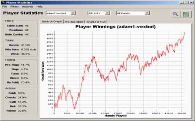
player analyzes their opponent’s strategy, and devises 1. Each player places 1 chip in the pot.
a best response. 2. Once a best response is calculated, 2. Each player is then presented with one card
it is incorporated into or replaces the current strategy from a (in this case 169 card) deck.
of the player. 3. The opposing player executes steps 1 3. One player is designated to start the betting
& 2 for themselves. 4. The whole process repeats (Player 1).
until a stable solution is achieved. Note that the ability 4. Player 1 makes a decision to bet, check, or
of fictitious play to solve a game is not guaranteed, for fold.
in some rare cases solution stability can not be 5. Player 2 then makes a decision to bet,
achieved. check/call, or fold.
6. The game ends when any player calls the
other’s bet, or when any player folds. The
maximum number of raises is 4.
7. After the betting sequence, the player not to
fold, or the player with the higher card wins
the pot.
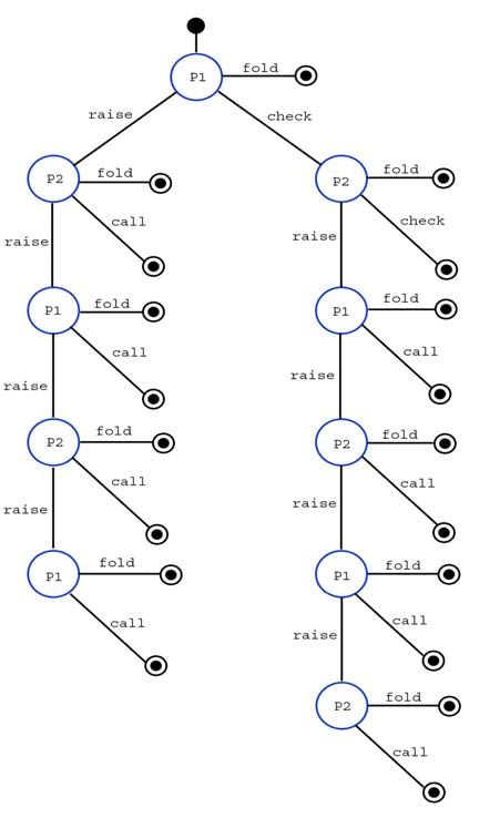
This simple poker variant was solved using fictitious
play, the solution of which is presented in Figure 2
with the terminal node connections removed.
Figure 1 - Game tree representation of One-Card
One-Round Poker
2.2.2 Solution to Simple Poker Variants Figure 2 - Optimal solution to One-Card One-
Using Fictitious Play Round poker.
Prior to a large attempted solution using fictitious
play, very basic poker games were constructed and
solved, one of which is presented here:
One-Card One-Round Poker (Figure 1):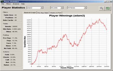
3 Abstractions                                            3.2.1 Bucketing/Grouping

3.1 Nature of the Problem of Poker                             Bucketing is an excellent and commonly used
                                                          abstraction technique that incurs minimal loss of
                                                          information, and yields large reduction in problem
     The game of 2-player Texas Hold’em is a
                                                          size. By grouping hands of similar value into buckets,
problem of size O(10^18) [2]. The sheer size of the
                                                          we can abstract entire groups of hands that can be
problem makes clear the intractability of computing a
                                                          played similarly into a single quantum. This method
perfect solution to the game, however there are several
                                                          is conceptually very similar to using perfect
methods available that allow a reduction from
                                                          isomorphs, for example, in our algorithm all 311
O(10^18) to size O(10^7). Though the problem has
                                                          million possible flop states are bucketed into 256
been reduced by a significant margin, its key
                                                          categories; hands such as: “2h 4d, 3c 5s 6s” (hand,
properties can be preserved through appropriate
                                                          table) and “2d 5c, 4h 6d 3h” would be bucked
abstraction, and a pseudo-optimal solution can be
                                                          together, and treated as having the same state. The
solved for this smaller, more manageable problem.
                                                          algorithm’s preflop domain contains 169 buckets, and
                                                          each of the three following round domains contain 256
                                                          buckets. This is a significant improvement from
                                                          previous solutions which used at most 6 or 7 buckets
                                                          to describe each domain [2].

 Figure 3 - Progression from Domain A to Domain              Figure 4 - Progression from Domain A to
 B through chance Node (magnitude 4). In a real              Domain B through a conversion matrix.
 game tree, the chance node magnitude would be
 between 45 and 120,000.
                                                          3.2.2 Chance Node Elimination

                                                               For fictitious play to be a viable solution method,
3.2 Game Tree Abstraction                                 a well-defined, tractable game tree must be
                                                          established. In the pure solution (not abstracted), the
     The purpose of using abstraction is to reduce the    tree can be represented as 4 tree domains (preflop,
size of the solution algorithm without modifying in the   flop, turn, and river), each of which having 10 nodes
underlying nature of the problem. In poker, there are     (with exception of preflop because of special game
available several methods of abstraction which do not     rules, having 8) (refer to Figure 1 for an example of a
detract at all from the solution, two of which are        single-domain tree). As a leaf node from one domain
position isomorphs (for the two cards in the hand, or     proceeds to the next domain (through a check/call
the three cards in the flop, position does not matter),   action in anything but the root of the domain),
and suit equivalence isomorphs (4s 5h in the hand         depending on the domain change, thousands of
preflop is equivalent to having 4c 5d, et al.). Using     subtrees must be formed from the movement (Figure
the available perfect isomorphs unfortunately does not    3). This structure becomes quickly unusable, for as
reduce the game size to a significant enough degree to    the tree continues to expand through chance nodes
yield the problem solvable given current techniques.      between domains, its size increases at a rapid
                                                          exponential rate.
In the solution presented, the problem regarding method produces a generic conversion that while
the exponential blow-up of the game tree size is being imperfect, shares the same statistical properties
addressed by eliminating chance nodes between as a tailor-made conversion distribution based on the
domains completely. Though removal does introduce specific game state. This method also has the benefit
error, the essence of the chance nodes are preserved of being faster to calculate on the fly, requires less
and replaced by conversion matrices which provide before-hand calculation, and requires less memory
similar function while reducing the exponential blow- overhead than the perfect transition discussed next.
up of the game tree (Figure 4). Using this strategy,
each leaf node has exactly one sub domain tree 3.2.3.2 Perfect Transition
associated with it. This produces a considerably
lighter game tree to solve, and with the chance nodes By calculating before-hand for every possible
removed from the solution, the problem is reduced to game-state its corresponding bucket, it is possible to
solving a tree with 6468 decision nodes instead of use this information on the fly to create a tailor-made
quite literally millions of billions of nodes. conversion matrix based on the game-state of Domain
A, and the game-state of Domain B. This approach
offers a great advantage in that it allows ‘perfect’
transitions between domains rather than a convincing
generic transition offered by a masking method. The
first of three issues invited by using this method is that
since there are so many possible game states, the
Figure 5 - Progression from Domain 1 with matrix must be created on the fly; reserving the
possible states {A,B,C,D} to Domain 2 with computational resources required to create these
possible states {a,b,c,d} using a conversion matrices slows down calculation considerably. The
matrix second issue is that the buckets for each game-state
Assumptions: must be known in advance (a task which depending on
P(A)+P(B)+P(C)+P(D) = 1 the problem size can easily be intractable). The last
P(a|x)+P(b|x)+P(c|x)+P(d|x) = 1 issue is that (in the case of the current implementation)
the buckets for these hundreds of millions of states,
once calculated, must reside in memory; using the data
off the hard drive at this time seems to be an
3.2.3 Transition Probabilities unattractive option for speed concerns.
Since the chance nodes have been completely
removed from the game tree, and a bucketing
approach is being used to represent states within each 4 Training an Optimal Player
domain, a method to convert buckets from a Domain A
to equivalent buckets in a Domain B requires a series Our algorithm which we refer to as Adam, was
of transition probabilities. This process can be trained using a technique based on Fictitious Play
accomplished with a conversion matrix, where each (section 2.2), described earlier; the premise behind the
column represents a bucket within Domain A, and training is that if two players who know everything
each row represents the corresponding probability that about each other’s playing style adapt their own styles
the Domain A bucket will translate into the Domain B long enough, their playing decisions will approach
bucket represented by the column number (Figure 5). optimality. This optimality is achieved in Adam by
These conversion matrices are expensive to compute, subjecting the decision tree to randomly generated
as each must be representative of the thousands of situations, analyzing how to play ‘correctly’ for the
chance nodes which they replace. specific situation (based on how we know we will play
and our opponent will play), and adapting the generic
3.2.3.1 Masking Transition solution slightly toward the correct action just
discovered. To solve two-player Texas Hold’em,
The first method explored, and one which proved hundreds of thousands of iterations of this basic
to work fairly well, was to create generic procedure need to be applied to every node of the
transformation probabilities, convert the buckets from decision tree before the solution suitably approaches
domain to domain, and then mask the converted optimal play.
bucket probabilities based on specific information
about the game-state of Domain B (Figure 6). This5 Playing Adam
Game theoretic solutions are distinguished in that
the strategies produced are randomized mixed
strategies; however though Adam is pseudo-optimal,
the strategies produced are not entirely mixed. The
decision tree represents a trimmed version of the
optimal decision tree (one which would include all
chance nodes between domains). Because of the
abstraction chosen, the flop, turn, and river domains
do not have a direct relationship with their optimal
cousin; however the preflop domain remains Figure 7. 20,000 hand performance against PsOpti.
unchanged even after the abstraction. This (winnings on the y-axis, hands played along x-axis)
dissimilarity between domains translates into different
approaches toward using the game tree in actual game
play. In evaluating preflop states, Adam is able to rely
on its preflop solution to provide approximate game-
theoretic optimal strategies, and in turn, Adam uses the
mixed strategies developed for preflop within its game
play. Post-flop, Adam can not rely on the generic
strategies developed through training to be suited for
current board conditions, and must use them solely for
reference to estimate future actions. Adam, given
current information then queries the sub tree from the
current decision node, and chooses the action which is Figure 8. 50,000 hand Performance against Vexbot.
assessed to have the highest value. (winnings on the y-axis, hands played along x-axis)
Both Figure 6 and Figure 7 represent separate
6 Experimental Results competitions against another pseudo-optimal
opponent. That our solution is able to consistently win
Adam was played in competition against two against this player suggests that the solution generated
algorithms created by a team of researchers from the by our algorithm is significantly closer to true
University of Alberta: PsOpti, a pseudo-optimal optimality.
solution, and Vexbot, a maximal algorithm. This
research group has released a software package called Figure 8 represents a competition between our
Poker Academy. A pseudo-optimal solution for Two- derived solution, and a maximal algorithm which is
Player Texas Hold’em was generated by our algorithm designed to find flaws in pseudo-optimal solutions.
was placed in competition with both PsOpti and The chart indicates that the maximal algorithm was
Vexbot via interfaces provided in their software. unable to find faults in our solution, and therefore
Figures 6-8 illustrate the results of the competition. consistently looses as the competition progresses.
This does not suggest that there are no flaws in our
solution; rather that the flaws are so small that the
maximal opponent is unable to detect and exploit
them.
7 Future Work
As processing power and memory capacity
increases, the abstractions used can be slowly weaned
from the problem, and more precise solutions may be
Figure 6. 20,000 hand performance against PsOpti. derived. We believe that increasing the current 256
(winnings on the y-axis, hands played along x-axis) buckets per round will not yield substantive benefits;
rather an approach that does not totally eliminatechance nodes, but replaces extensive chance nodes
(such as preflop to flop with 117 thousand branches)
with a smaller group of abstracted ‘bucketed’ branches
may lead to solutions far closer to optimality.
8 Conclusion
The expansion beyond minimax approachable
games such as Chess and Backgammon has taken
computer science and game theory into new areas of
research. However, these new problems require
different methods of solution then perfect information
games, and presented is one such method applied to a
domain representative of many real-world problems.
Using proper abstraction techniques it is shown that
fictitious play can and succeed in approaching Nash
Equilibria in complex game theoretical problems such
as full-scale poker.
Acknowledgements
Thanks go to Dr. C.-C. Chan for helping me
publish this work. Thanks are also extended to the
Department of Computer Science at the University of
Akron for supporting my research efforts.
References
[1] Brown, G.W. Iterative Solutions of Games by
Fictitious Play. In Activity Analysis of
Production and Allocation, T.C. Koopmans
(Ed.). New York: Wiley.
[2] D. Billings, N. Burch, A. Davidson, R. Holte, J.
Schaeffer, T. Schauenberg, and D. Szafron.
Approximating Game-Theoretic Optimal
Strategies for Full-scale Poker. Proceedings
of the 2003 International Joint Conference on
Artificial Intelligence.You can also read