Visualization of bat "echo space" using acoustic simulation

Visualization of bat “echo space” using acoustic
simulation
Yu Teshima (  yuteshima18@gmail.com )
 Doshisha University https://orcid.org/0000-0002-1202-470X
Yasufumi Yamada
 Hiroshima University
Takao Tsuchiya
 Doshisha University
Olga Heim
 Doshisha University
Shizuko Hiryu
 Doshisha University

Article

Keywords: echolocation, bats, ight navigation

Posted Date: June 2nd, 2021

DOI: https://doi.org/10.21203/rs.3.rs-512467/v1

License:   This work is licensed under a Creative Commons Attribution 4.0 International License.
Read Full License

1 Visualization of bat “echo space” using acoustic simulation
 2
 3

 4 Abstract
 5 Behavioral experiments with acoustic measurements have revealed the intriguing

 6 strategies of flight navigation and the use of ultrasound by echolocating bats in various

 7 environments. However, the echolocation behavior of bats has not been thoroughly

 8 investigated in regard to the environment they perceive via echolocation because it is

 9 technically difficult to measure all the echoes that reach the bats during flight, even with

10 the conventional telemetry microphones currently in use. Therefore, we attempted to

11 reproduce the echoes of bats during flight by combining acoustic simulation and

12 behavioral experiments with acoustic measurements. As a result, we visualized the

13 spatiotemporal changes in the echo incidence points detected by bats during flight, which

14 enabled us to investigate the “echo space” revealed through echolocation. In addition, we

15 could observe how the distribution of visualized echoes concentrated at the obstacle

16 edges after the bats became more familiar with their environment. Furthermore, our

17 results indicate that the direction of preceding echoes affects the turn rates of the bat's

18 flight path, revealing their original echolocation behavior.

19

20 Introduction

21 Humans rely heavily on vision as a result of their exceptionally high visual acuity
 1
22 . This superiority of human vision has guided the direction of technological development
 1

23 in recent years. For instance, image recognition and simultaneous localization and

24 mapping technologies using stereo and monocular cameras, such as automated driving,

25 have advanced rapidly, particularly in combination with deep learning 2,3. The accuracy

26 of image processing technology has significantly improved in recent years and hence, is

27 an important technological element in the field of sensing.

28 In contrast to humans, other animals optimize their behavior in weak vision or

29 grasp their environment with sensory organs other than vision. For instance, echolocating

30 bats mainly operate in the dark (e.g., caves and at night) where they cannot rely on vision

31 but can perceive their environment via acoustic sensing using ultrasound 4. Knowledge

32 about a bat’s sonar system has been accumulated through various experiments that, for

33 instance, determined how bats alter ultrasound characteristics in response to various

34 situations 5–7 and quantitatively measured the high acoustic acuity of the bat’s sonar 8,9.

35 Using the basic principle of sensing with one transmitter and two receivers, bats can

36 estimate object distance based on the echo delay time 10,11 and can localize objects by

37 relying on the information difference between the echoes reaching the left and right ears
 12
38 . This simple principle is also commonly used in the field of engineering, so that the

39 bat’s sonar has been proposed as a model for object localization 13 and obstacle avoidance

40 algorithms 14,15, and is practically applied to an autonomous robot 16–18. Ultrasonic

41 sensing has been widely utilized to perceive our environment in a simple manner, as it is

42 relatively inexpensive to produce and handles a much smaller amount of data compared

43 to methods based on vision. Further improvements in acoustic sensing technology can be

44 expected if knowledge of bat biosonar systems can be incorporated into the field of

45 engineering.
 2

46 Previous studies on the bats’ behavior suggest that information about space or an

47 object can differ depending on whether it was acquired via vision or echolocation. For

48 instance, bats are known to collide with a smooth surface wall during flight 19 in cases

49 where pulses are transmitted at a certain angle to the wall so that no echo is returned. In

50 other words, a smooth surface wall is perceived as an empty space by bats, although the

51 same wall can be perceived visually. In another example, nectar-feeding bats

52 (Glossophaga soricina) were able to find the feeder in approximately half the time when

53 the dish-shaped leaves of Marcogravure ebenezer were attached to the feeder. The dish-

54 shaped leaves reflect echoes of similar intensity at wide angles and consequently make it

55 easier for the bats to detect it 20. These examples demonstrate how we can imagine the

56 difference in perception based on sound and vision.

57 Since humans are highly focused on visual perception, one effective approach to

58 better understand how the acoustic perception of bats works can be to visualize the world

59 as perceived by sound. Thus it is necessary to focus on the echoes received by the bats

60 rather than on the emitted pulses. Therefore, as one of the first studies, we aim at

61 investigating the echolocation strategy of bats based on the information received from

62 echoes. Since, it is difficult to measure all the echoes reaching both ears of a bat during

63 flight, even with a conventional telemetry microphone 21 or an onboard acoustic logger 22,

64 we propose a new approach. In particular, we propose to combine information from

65 behavioral experiments (e.g. flight paths, emitted pulse directions) with acoustic

66 simulation to estimate the echoes that reach the right and left ears of a bat in flight. Based

67 on this acoustic simulation, we can reconstruct the locations and directions of echoes and

 3

68 thus visualize the “echo space” as the entirety of these echoes. In addition, we examine

69 how the echo space changes as the bats become more familiar with their environment.

70

71 Results

72 Bats (Rhinolophus ferrumequinum nippon) were allowed to fly repeatedly through

73 a course with acrylic plates as obstacles, and their flight trajectories and pulse

74 information (direction, intensity, and timing of emission) were measured 23. The same

75 obstacle course layout as in the behavioral experiment was constructed as a two-

76 dimensional acoustic simulation space, and acoustic simulation was performed using the

77 finite-difference time-domain (FDTD) method. With the information on the positions and

78 pulses of the bats acquired in the behavioral experiment, we could determine the echoes

79 that reached the positions of the right and left ears of the bats in flight in the simulation.

80 Based on the left and right echo delay times we then estimated the echo incidence points

81 and visualized them as the echo space (Supplementary Movie S1).

82 Spatial learning affects echo incidence point distribution

83 The echo incidence points were mostly concentrated near the inner edge of the

84 obstacle wall (Fig. 1 & 2A,). Therefore, we selected those echo incidence points that

85 were located within the inner half of the obstacle wall to investigate the effect of spatial

86 learning on their distribution. We modeled the distance from the echo incidence points to

87 the inner edge of the walls using generalized linear mixed effect models. We found that

88 echo incidence points after spatial learning were located closer to the inner edge than

89 before spatial learning (contrastFirst/Last: ratio=1.2 ±0.07 SE, df=1053, t-ratio=3.6,

 4

90 p

a b

101
102 Figure 2. Distribution of echo incidence points on obstacle walls during the first and

103 last flight. a The histogram shows the probability of echo incidence points being located

104 at various distances to the inner edge of the obstacle (acrylic walls) during the first and

105 last flight. b Box plots summarize data on the distances between echo incidence points

106 and the inner edge within the inner half of obstacle walls for the first and last flight, while

107 the black whisher plots represent model-related means (black circle) and associated 95%

108 confidence intervals. These results are based on a model that fit the data well (based on

109 residual plots) and that explained significantly more variance than its null model

110 (χ2=12.95, df=1, p

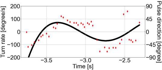
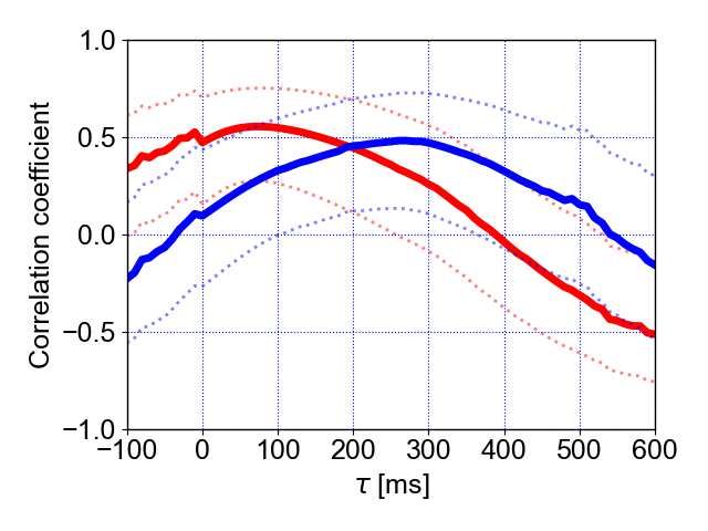
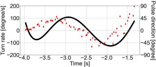
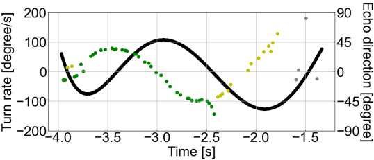
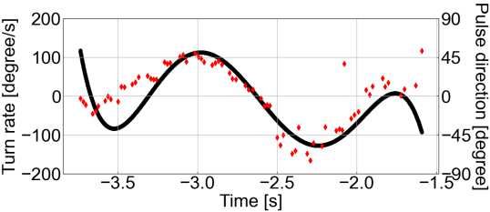
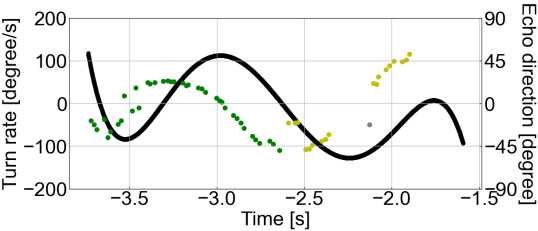
117 plotted individual-specific time-series (Fig. 3A, B, see Supplementary Figs. S2, S3 for

118 data on all the individuals) and found that although both, pulse and echo direction change

119 precedes the turn rate change, the echo direction changes more smoothly and precedes the

120 turn rate change with a larger time lag than the pulse direction (Fig. 4A). To test this

121 observation statistically and to test for any effects of spatial learning, we determined the

122 individual-specific time delay τmax at which a pulse or an echo direction, respectively, are

123 maximally correlated to a turn rate. After modeling τmax as a function of the bat’s

124 experience in interaction with the type of direction (echo or pulse), we found that, during

125 the first flight, pulse and echo direction changes preceded the turn rate change at 186 ±

126 54 ms and 377 ± 54 ms, respectively. In this case, the echo direction change tended to

127 precede the turn rate with a larger time lag than that of the pulse direction change

128 (contrastEcho/Pulse: ratio=191 ± 68 SE, df=18, t-ratio=2.8, p=0.069, Fig. 4B). During the

129 last flight, the time lags between the pulse and echo direction change and the turn rate

130 change decreased slightly to 74 ± 54 ms and 233 ± 54 ms, respectively (Fig. 4B). Also,

131 the difference between time lags of echo and pulse direction changes decreased slightly

132 (contrastEcho/Pulse: ratio=159 ± 68 SE, df=18, t-ratio=2.3, p=0.19, Fig. 4B). Based on the

133 inter-peak time lag difference between echo and pulse direction of 191 ms (= 377 ms –

134 186 ms) during the first flight, we estimate that an echo direction might affect the

135 direction of the fifth (4.6 ± 1.9) pulse following that echo. In contrast, we estimate that

136 the echo direction possibly affects the direction of the third (3.0 ± 1.6) pulse during the

137 last flight.

 7

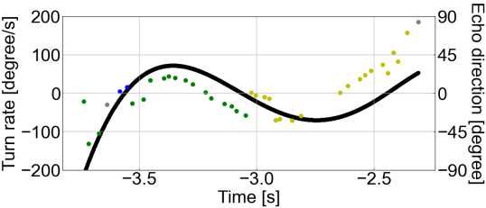
a b

 Bat A

 Bat B

 Bat C

138
139 Figure 3. Time series plots of the pulse direction and turn rate, and echo direction

140 and turn rate in the first flight. a Time series plot of the pulse direction (red rhombus

141 plot) and turn rate (black solid line) in the first flight for each bat. b Time series plot of

142 the echo direction (plotted) and turn rate (solid black line) for each bat in the first flight.

143 The echo direction plot shows the echo incidence points with the highest sound pressure

144 generated by a single pulse. The color of the echo direction plot depends on the obstacle

145 (acrylic plate) on which the echo incidence is localized: blue indicates the first acrylic

146 plate, green the second acrylic plate, yellow the third acrylic plate, and gray the echo

147 source that was not localized on the obstacle.

 8

a First flight
 b

 Last flight

148
149 Figure 4. Correlation coefficients between the pulse direction and turn rate and

150 between the echo direction and turn rate for the first and last flight. a Correlation

151 coefficients between the pulse direction and turn rate (solid red line) and between the

152 echo direction and turn rate (solid blue line). The dotted lines represent 95% confidence

153 intervals. b The statistical comparison of individual-specific time lag data shows means

154 (circles) and 95% confidence intervals (whiskers) for echo and pulse directions during the

155 first and last flight. These results are based on a model that fit the data well (based on

156 residual plots) and that explained significantly more variance than its null model

157 (parametric bootstrap test, stat=16.0, df=3, p=0.007). The effect of the spatial-learning-

158 factor in interaction with the type of information (echo or pulse) was found to be not

159 significant (χ2type-II-Wald=0.12, df=1, p=0.7) while the single effects showed a clear effect
 9

160 (flight (first vs. last): χ2type-II-Wald=7.07, df=1, p=0.008; information (echo vs. pulse): χ2type-

161 II-Wald=13.25, df=1, p

183 data demonstrate how different information from visually perceived objects can be to

184 information perceived via sound. Consequently, for understanding the behavior of a bat

185 flying through an obstacle course, not only the direction of emitted pulses but also the

186 location of generated echo incidence points should be considered at the same time.

187 In a previous study, it was shown that the number of pulses emitted during flight

188 decreased with progressing spatial learning 23, which appears to be in agreement with our

189 finding that the echo space also changed between the first and last flight. After bats have

190 become familiar with the obstacle course, the echo incidence points are concentrated at

191 the edge of the target, which is important for grasping the obstacle space. As a result, bats

192 seem to reduce the number of pulses necessary for collecting this information. Bats are

193 known to have spatial and shape memory 27–30; therefore, by matching received

194 information with the memorized space, it could be possible to obtain the necessary

195 information about the space using a small number of pulses.

196 The bats are affected by not only the pulse direction but also the echo direction, and

197 the time of influence is earlier in the echo direction than in the pulse direction. This is a

198 natural result, considering that bats change the characteristics of the following pulse

199 based on information of the previous echoes. For instance, previous studies have

200 suggested that the Doppler shift compensation behavior is based on the echoes of the

201 previous one to three pulses 31, and in the bat's target direction anticipation behavior, the

202 model best matches the measured data when the target velocity is estimated from the

203 echoes of the previous five pulses 32. In the present study and during the first flight, we

204 found a positive correlation peak of the pulse direction that preceded the turn rate change

205 by 186 ms, which is similar to the time lag obtained in an obstacle environment in a
 11

206 previous study 33. In contrast, the echo direction change preceded the turn rate change by

207 377 ms (Fig. 4A) which suggests that the effect of the pulse direction on the turn rate may

208 be a secondary result of the echo direction affecting the turn rate. Based on our results we

209 estimated that the echo direction possibly affects the direction of approximately the fifth

210 pulse during the first flight, which is consistent with the results of the above-mentioned

211 study 31,32. In comparison the first flight, we found that the echo direction possibly affects

212 the direction of earlier pulses during the last flight. Thus bats might be able to reduce the

213 time required to determine the turn rates and pulse directions after the arrival of echoes

214 when they have become familiar with their surroundings.

215 In this study, we found that bats tend to focus more on the inner edges of obstacles

216 after spatial learning. Therefore, it is important to identify the edges of objects for object

217 recognition and avoidance. In the case of object identification using images from

218 cameras, there are many algorithms that can be used for edge extraction, such as the

219 Scale-Invariant Feature Transform 34. In contrast, in sound object recognition, diffracted

220 waves are reflected from the edges as echoes in addition to a direct wave (see

221 Supplementary Fig. S4 and Supplementary Movie S1). In other words, in sound-based

222 object recognition, solely information from the direct wave and diffracted wave from the

223 edge is contained in the echoes. In contrast to object recognition by images, sound-based

224 methods may be more efficient because only minimal information is required. In this

225 study, we simulated the echoes and visualized echo space based on an engineering

226 approach; however, it is necessary to reproduce the actual process in bats more precisely

227 in the future, so that we can obtain a clearer understanding of the space perceived by bats.

228 For instance, we should include the directivity of the ear position by introducing the
 12

229 head-related transfer function (HRTF) of the bat, including its ears, in the acoustic

230 simulation space and a moving source to reflect the effect of the Doppler shift during

231 flight to obtain more detailed spatial information. In addition, a bat auditory processing

232 algorithm should be introduced into the post-echo processing such as the spectrogram

233 correlation and transformation (SCAT) model 35–37. We believe that this approach of echo

234 simulation is a useful first step towards elucidating the perception space by bats.

235

236 Methods

237

238 Study species

239 Seven adult Japanese greater horseshoe bats (Rhinolophus ferrumequinum nippon,

240 three males and four females) were used for the behavioral experiment. The bats of this

241 species emit pulses consisting of a short initial FM component (iFM), a constant

242 frequency component (CF), and a terminal FM component (tFM). These pulses are

243 accompanied by overtones. Among the overtones, the second overtone, which has a CF

244 component of approximately 68–70 kHz, has the highest sound pressure 21.

245

246 Experimental setup and procedure

247 The experiment was conducted in a corridor [4.5 m (L) × 1.5 m (W)] bordered by

248 chains within a flight chamber [9 m (L) × 4.5 m (W) × 2.5 m (H)]. Three acrylic panels [1

249 m (W) × 2 m (H)] were placed in the corridor next to the chain-walls, alternating on the

250 left and right side, with each panel being spaced 1 m apart from each other

251 (Supplementary Fig. S5). The seven bats were allowed to fly one after the other from the
 13

252 starting position through the obstacle course to a net behind the starting position 12 times.

253 At the time of their first flight, they were completely unfamiliar with the obstacle course.

254 Also, the experimenter carried each bat to the starting position of the flight while

255 covering the bat with his hands to prevent it from collecting information about its

256 surroundings. After a bat has flown through the course once, the experimenter

257 immediately captured the bat using a 50 cm × 50 cm insect net. Then the bat was allowed

258 to drink water from a plastic pipette and was brought back to the starting point by the

259 experimenter who was covering them with their hands while carrying. During the

260 experiment, only infrared lights were used in the flight chamber. Two high-speed video

261 cameras (MotionPro X3; IDT Japan, Inc., Tokyo, Japan; 125 frames per second) recorded

262 the flight paths of the bats, and microphones arranged in an array around the flight

263 chamber recorded the emitted pulses of the bats to calculate the direction of pulse

264 emission. We also calculated the pulse emission timing of the bats by measuring the

265 pulses they emitted using a telemetry microphone attached to the bat's head. The methods

266 were performed in accordance with the Principles of Animal Care (publication no. 86-23,

267 revised 1985) issued by the National Institute of Health in the USA and regulations and

268 pre-approved by the Animal Experiment Committee of Doshisha University. Please refer

269 to the publication of Yamada et al. 23 for further methodological details.

270

271 Finite-difference time-domain (FDTD) method

272 We used the two-dimensional FDTD method to simulate the echoes that return to

273 the positions of the right and left ear of bats during their flight. The FDTD method is one

274 of the numerical methods developed by Yee to solve Maxwell's equations, which are the
 14

275 governing equations of electromagnetic waves 38. It has been widely used in the field of

276 acoustics since Madariaga adapted it for elastic waves 39. The method uses the governing

277 equations of motion and the continuity of sound pressure as given in equations [1] and

278 [2].

279 + ∙ = [ ]
 
280 + = [ ]
 
281 where p is the sound pressure, u is the particle velocity vector, is the medium density,

282 and is the speed of sound. The following equations are obtained by discretizing the

283 above governing equations on a staggered grid.

 ∆ + +
 
 +
 
 +
 
284 + 
 , = , − ( − + − ) [ ]
 ∆ + , 
 
 − , 
 
 , +
 
 , −
 
 + − ∆ 
285 
 = 
 − ( − , ) [ ]
 
 + , 
 
 + , 
 
 ∆ + , 

 + − ∆ 
286 
 = 
 − ( − , ) [ ]
 
 + , 
 
 + , 
 
 ∆ + , 

287 where ∆ is the grid interval and ∆ is the time resolution. The terms , , , , and , 

288 are the sound pressure and particle velocity at a position (x, y) = (i∆, j∆) and time t = n∆ ,

289 respectively. The sound propagation is calculated by alternately solving equations [3],

290 [4], and [5]. In addition, because FDTD is a time- and not a frequency-domain acoustic

291 simulation, diffuse attenuation is included, while the absorption attenuation is not.

292

293 Visualization of echo incidence points

 15

294 Simulation space set-up

295 In the behavioral experiment, the obstacle walls (acrylic plates) were reaching from

296 the floor to the ceiling, so that bats avoided them by changing their horizontal flight path.

297 To obtain the direction of the bat’s pulse emission, a microphone array was placed at a

298 height of 1.2 m. To recreate this setup in our simulation space, we created a two-

299 dimensional space (x–y) on the height level of the array microphones (z = 1.2 m). The

300 FDTD simulation space was located inside the corridor (4.5 m × 1.5 m) as shown in

301 Supplementary Fig. S6A, and the absorption boundary condition was the Mur second-

302 order boundary condition 40. As presented in Table S1, the Courant–Friendrichs–Lewy

303 (CFL) number was 0.57. The spatial resolution (dx) was 0.3 mm. And the densities of air

304 and acrylic were 1.29 kg/m3 and 1.18 kg/m3, with a bulk modulus of 142.0×103 Pa and

305 8.79×109 Pa, respectively.

306

307 Echo simulation

308 To simulate the echoes that returned to the position of the bats' ears, we used

309 information on the bats’ pulse emission position and direction obtained from the

310 behavioral experiment. A sinc function signal with a wide frequency band and high time

311 resolution were used in the simulation space as the emitted pulse. It was flat up to 110

312 kHz and the duration was 0.073 ms (Supplementary Fig. S6B). The sinc function signal

313 was emitted from two source positions (simulating the bat’s nostrils), which were set at

314 1.25 mm each on the left and right side from a given pulse emission position and in the

315 direction of emission which was both obtained from the behavioral experiment

316 (Supplementary Fig. S7A; note that 1.25 mm is based on the half wavelength of the CF2
 16

317 frequency of R. ferrumequinum nippon (68 kHz)) 41,42. Receiver positions (simulating the

318 bat’s ears) of the returning echoes in the simulation were set at 10 mm left and right from

319 the pulse emission points (note that 10 mm is based on the distance between the ears of R.

320 ferrumequinum nippon) (Supplementary Fig. S7A). In the simulation, the impulse

321 responses (echoes) at the two receiver positions were calculated using the FDTD method.

322 Then, the bat’s pulse was convolved with these impulse responses to obtain echoes. The

323 bat’s pulses in the simulation were the downward FM components created up to the third

324 harmonic, which has been reported to be used for distance discrimination 43. The

325 downward FM component has a duration of 2 ms and the first harmonic decreases

326 linearly from 34 kHz to 25 kHz, corresponding to the terminal FM component of the

327 echolocation pulse in R. ferrumequinum nippon (Supplementary Fig. S7B). The first and

328 third harmonics were set to a sound pressure level of -40 dB based on the second

329 harmonic 44. The sampling frequency was 2 MHz (1 / dt).

330

331 Calculation of echo incidence points

332 Bats estimate the distance to an object based on the time delay between the emitted

333 pulse and the echoes 10,11. In the simulation, this echo delay was calculated by cross-

334 correlating the simulated left and right echoes with the bat’s pulses. The peak value of the

335 autocorrelation of the pulse was normalized, and the peak time above the threshold of the

336 cross-correlating signal was extracted for the left and right echoes (Supplementary Fig.

337 S8). The threshold value was set to 0.02 to detect almost all the peaks. The left and right

338 peak times were matched within a window of the maximum time difference between the

 17

339 two receiving points (2.5 mm / 340 m/s = 7.4 µs), and combinations of the left and right

340 peak times ([tr, tl]) were obtained. The echo incidence points ((xecho, yecho)) were then

341 calculated by solving the following two elliptic equations determined by the calculated

342 peak times using the pulse emission positions obtained in the behavioral experiments

343 (i.e., the centers of the two source positions in the simulation) and the left and right

344 receiver positions in the simulation space as the focal points. The pulse emission position

345 was set to y = 0 and the direction of pulse emission was set to x = 0.

 ( − ) ( − ) 
346 + = [ ]
 
 ( − ) ( − ) 
347 + = [ ]
 
 ∙ 
348 = , = √ − ( − ) 
 
 ∙ 
349 = , = √ − ( − ) 
 
350 where xr0 is the center position between the pulse emission position and the right receiver

351 position, and xl0 is the center position between the pulse emission position and the left

352 receiver position (see Supplementary Fig. S9). An animation of the process of echo

353 incidence point visualization using acoustic simulation is shown in Supplementary Movie

354 S1.

355

356 Statistical Analysis

357 Effect of spatial learning on the echo incidence point distribution

358 We were interested in testing whether the positions of echo incidence points on the

 18

359 obstacle walls changed depending on the spatial learning status of the bats (first vs. last

360 flight). Since the bat’s task in the behavioral experiment was to avoid the inner sides of

361 the obstacle walls, we considered those echo incidence points that were located on the

362 inner half of the walls and calculated the distance of these points to the inner edge. We

363 modeled this data as a function of the bat’s spatial learning status (first vs. last flight)

364 using generalized linear mixed effect models (function glmmTMB, package

365 glmmTMB_1.0.2.1) 45 assuming a negative binomial error distribution (nbinom1) due to

366 overdispersion. Because several echo incidence points can result from one pulse and

367 several pulses were used per bat, we included a random effect with a pulse-ID nested

368 within the bat-ID. The quality of the model fit was graphically examined (function in

369 package DHARMa_0.3.3.0) 46 and its overall significance was determined by comparing

370 it to the respective null model that contains only the random effect via a χ2-test (function

371 anova in stats) 47. The significance of the factor coding for the bat’s experience was

372 derived from a type-II-Wald- χ2-test (function anova, package car_3.0-10) 48 while the

373 factor-levels were compared based on least-square-means (function lsmeans, package

374 emmeans_1.5.4) 49. The statistical significance level was set at p = 0.05.

375

376 Effects of spatial learning on flight path planning

377 We calculated the turn rate at 1 ms intervals from the acquired flight paths. The turn

378 rate is the time derivative of the flight path. To investigate the relationship between the

379 turn rate and the pulse and echo direction, respectively, we shifted the turn rate data by a

380 time lag of τ in 10 ms steps from -100 ms (to the left) up to + 600 ms (to the right)

381 relative to the pulse and echo direction, respectively, and calculated the corresponding
 19

382 correlation coefficients. The 95% confidence intervals for the correlation coefficients

383 were determined by a Fisher transformation of the correlation coefficients to the

384 following

385 ranges
 
386 ± / [ ]
 √ − 

387 where n represents the number of data and / is 1.96 for 95% confidence interval.

388 Then, we extracted the τ-values that were associated with the highest correlation

389 coefficients for each bat and each category (first vs. last flight) and modeled them on the

390 scale of seconds as a function of the degree of spatial learning (first vs. last flight) in

391 interaction with the factor describing the type of information used by the bat (echo vs.

392 pulse) using linear mixed effect models (function lmer, package lme4_1.1-26) 50. We

393 added the bat-ID as a random effect to the model due to the repeated sampling of the

394 same individuals. The quality of the model fit, the significance of factors within the

395 model, and the comparisons between factor-levels were conducted using the same

396 functions as mentioned above. The overall model significance was tested against the

397 respective null model using parametric bootstrapping (function PBmodcomp, package

398 pbkrtest_0.5-1.0) 51.

399

400 Data Availability

401 The data used in this study and the code used in the analysis are available at

402 GitHub,

403 https://github.com/tsmyu/Visualization_of_bat_echo_space_by_using_acoustic_simulatio

 20

404 n.

405 References
406
407 1. Caves, E. M., Brandley, N. C. & Johnsen, S. Visual Acuity and the Evolution of
408 Signals. Trends Ecol. Evol. 33, 358–372 (2018).
409 2. Taketomi, T., Uchiyama, H. & Ikeda, S. Visual SLAM algorithms: A survey from
410 2010 to 2016. IPSJ Transactions on Computer Vision and Applications vol. 9
411 (2017).
412 3. Gordon, A., Li, H., Jonschkowski, R. & Angelova, A. Depth from videos in the
413 wild: Unsupervised monocular depth learning from unknown cameras. in
414 Proceedings of the IEEE International Conference on Computer Vision (2019).
415 4. Griffin, D. R. & Lindsay, R. B. Listening in the Dark. Phys. Today 12, 42–42
416 (1959).
417 5. Surlykke, A. & Moss, C. F. Echolocation behavior of big brown bats, Eptesicus
418 fuscus , in the field and the laboratory . J. Acoust. Soc. Am. 108, 2419–2429 (2000).
419 6. Moss, C. F. & Surlykke, A. Auditory scene analysis by echolocation in bats. J.
420 Acoust. Soc. Am. 110, 2207–2226 (2001).
421 7. Hiryu, S., Bates, M. E., Simmons, J. A. & Riquimaroux, H. FM echolocating bats
422 shift frequencies to avoid broadcast-echo ambiguity in clutter. Proc. Natl. Acad.
423 Sci. U. S. A. 107, 7048–7053 (2010).
424 8. Bates, M. E., Simmons, J. A. & Zorikov, T. V. Bats use echo harmonic structure to
425 distinguish their targets from background clutter. Science (80-. ). 333, 627–630
426 (2011).
427 9. Simmons, J. A. et al. Acuity of horizontal angle discrimination by the echolocating
428 bat, Eptesicus fuscus. J. Comp. Physiol. □ A 153, 321–330 (1983).
429 10. Simmons, J. A. The resolution of target range by echolocating bats. J. Acoust. Soc.
430 Am. 54, 157–173 (1973).
431 11. Wohlgemuth, M. J., Luo, J. & Moss, C. F. Three-dimensional auditory localization
432 in the echolocating bat. Curr. Opin. Neurobiol. 41, 78–86 (2016).
433 12. Aytekin, M., Grassi, E., Sahota, M. & Moss, C. F. The bat head-related transfer
434 function reveals binaural cues for sound localization in azimuth and elevation. J.
435 Acoust. Soc. Am. 116, 3594–3605 (2004).
436 13. Kuc, R. Sensorimotor model of bat echolocation and prey capture. J. Acoust. Soc.
437 Am. 96, 1965–1978 (1994).

 21

438 14. Vanderelst, D., Holderied, M. W. & Peremans, H. Sensorimotor Model of
439 Obstacle Avoidance in Echolocating Bats. PLoS Comput. Biol. 11, 1–31 (2015).
440 15. Steckel, J. & Peremans, H. BatSLAM: Simultaneous Localization and Mapping
441 Using Biomimetic Sonar. PLoS One 8, (2013).
442 16. Yamada, Y. et al. Ultrasound navigation based on minimally designed vehicle
443 inspired by the bio-sonar strategy of bats. Adv. Robot. 33, 169–182 (2019).
444 17. Eliakim, I., Cohen, Z., Kosa, G. & Yovel, Y. A fully autonomous terrestrial bat-
445 like acoustic robot. PLoS Comput. Biol. 14, e1006406 (2018).
446 18. Mansour, C. B., Koreman, E., Steckel, J., Peremans, H. & Vanderelst, D.
447 Avoidance of non-localizable obstacles in echolocating bats: A robotic model.
448 PLoS Comput. Biol. 15, e1007550 (2019).
449 19. Greif, S., Zsebok, S., Schmieder, D. & Siemers, B. M. Acoustic mirrors as sensory
450 traps for bats. Science (80-. ). 357, 1045–1047 (2017).
451 20. Simon, R., Holderied, M. W., Koch, C. U. & Von Helversen, O. Floral acoustics:
452 Conspicuous echoes of a dish-shaped leaf attract bat pollinators. Science (80-. ).
453 333, 631–633 (2011).
454 21. Hiryu, S., Shiori, Y., Hosokawa, T., Riquimaroux, H. & Watanabe, Y. On-board
455 telemetry of emitted sounds from free-flying bats: Compensation for velocity and
456 distance stabilizes echo frequency and amplitude. J. Comp. Physiol. A Neuroethol.
457 Sensory, Neural, Behav. Physiol. 194, 841–851 (2008).
458 22. Cvikel, N. et al. On-board recordings reveal no jamming avoidance in wild bats.
459 Proc. R. Soc. B Biol. Sci. 282, (2015).
460 23. Yamada, Y. et al. Modulation of acoustic navigation behaviour by spatial learning
461 in the echolocating bat Rhinolophus ferrumequinum nippon. Sci. Rep. 10, 1–15
462 (2020).
463 24. Ghose, K. & Moss, C. F. Steering by hearing: A bat’s acoustic gaze is linked to its
464 flight motor output by a delayed, adaptive linear law. J. Neurosci. 26, 1704–1710
465 (2006).
466 25. Land, M. F. Eye movements and the control of actions in everyday life. Prog.
467 Retin. Eye Res. 25, 296–324 (2006).
468 26. Danilovich, S., Shalev, G., Boonman, A., Goldshtein, A. & Yovel, Y.
469 Echolocating bats detect but misperceive a multidimensional incongruent acoustic
470 stimulus. Proc. Natl. Acad. Sci. 202005009 (2020) doi:10.1073/pnas.2005009117.
471 27. Ulanovsky, N. & Moss, C. F. Hippocampal cellular and network activity in freely
472 moving echolocating bats. Nat. Neurosci. 10, 224–233 (2007).

 22

473 28. Toledo, S. et al. Cognitive map-based navigation in wild bats revealed by a new
474 high-throughput tracking system. Science (80-. ). 369, 188–193 (2020).
475 29. Barchi, J. R., Knowles, J. M. & Simmons, J. A. Spatial memory and stereotypy of
476 flight paths by big brown bats in cluttered surroundings. J. Exp. Biol. 216, 1053–
477 1063 (2013).
478 30. Yu, C., Luo, J., Wohlgemuth, M. & Moss, C. F. Echolocating bats inspect and
479 discriminate landmark features to guide navigation. J. Exp. Biol. 222, (2019).
480 31. Gaioni, S. J., Riquimaroux, H. & Suga, N. Biosonar behavior of mustached bats
481 swung on a pendulum prior to cortical ablation. J. Neurophysiol. 64, 1801–1817
482 (1990).
483 32. Salles, A., Diebold, C. A. & Moss, C. F. Echolocating bats accumulate information
484 from acoustic snapshots to predict auditory object motion. Proc. Natl. Acad. Sci.
485 202011719 (2020) doi:10.1073/pnas.2011719117.
486 33. Falk, B., Jakobsen, L., Surlykke, A. & Moss, C. F. Bats coordinate sonar and flight
487 behavior as they forage in open and cluttered environments. J. Exp. Biol. 217,
488 4356–4364 (2014).
489 34. D.G.Lowe. Distinctive image features from scale-invariant keypoints. Int. J.
490 Comput. Vis. 60, 91–110 (2004).
491 35. McMullen, T. A., Simmons, J. A. & Dear, S. P. A computational model of echo
492 processing and acoustic imaging in frequency-modulated echolocating bats: The
493 spectrogram correlationand transformation receiver. J. Acoust. Soc. Am. 94, 2691–
494 2712 (1993).
495 36. Ming, C., Bates, M. E. & Simmons, J. A. How frequency hopping suppresses
496 pulse-echo ambiguity in bat biosonar. Proc. Natl. Acad. Sci. U. S. A. 117, 17288–
497 17295 (2020).
498 37. Ming, C., Haro, S., Simmons, A. M. & Simmons, J. A. A comprehensive
499 computational model of animal biosonar signal processing. PLOS Comput. Biol.
500 17, e1008677 (2021).
501 38. Yee, K. S. Numerical solution of initial boundary value problems involving
502 Maxwell’s equations in isotropic media. IEEE Trans. Antennas Propag. 14, 302–
503 307 (1966).
504 39. Madariaga, R. Dynamics of an expanding circular fault. Bull. Seism. Soc. Am. 66,
505 639–666 (1976).
506 40. Mur, G. Absorbing boundary conditions for the finite-difference approximation of
507 the time-domain electromagnetic-field equations. 377–382 (1981).

 23

508 41. Strother, G. K. & Mogus, M. Acoustical Beam Patterns for Bats: Some Theoretical
509 Considerations. J. Acoust. Soc. Am. 48, 1430–1432 (1970).
510 42. Hartley, D. J. & Suthers, R. A. The sound emission pattern and the acoustical role
511 of the noseleaf in the echolocating bat, Carollia perspicillata. J. Acoust. Soc. Am.
512 82, 1892–1900 (1987).
513 43. Suga, N. The Extent to Which Biosonar Information Is Represented in the Bat
514 Auditory Cortex. in Dynamic Aspects of Neocortical Function 315–373 (John
515 Wiley & Sons, 1984).
516 44. Hartley, D. J. & Suthers, R. A. The acoustics of the vocal tract in the horseshoe bat,
517 Rhinolophus hildebrandti. J. Acoust. Soc. Am. 84, 1201–1213 (1988).
518 45. Brooks, M. E. et al. glmmTMB balances speed and flexibility among packages for
519 zero-inflated generalized linear mixed modeling. R J. 9, 378–400 (2017).
520 46. Hartig, F. DHARMa: Residual Diagnostics for Hierarchical (Multi-Level / Mixed)
521 Regression Models. (2020).
522 47. R Core Team. R: A Language and Environment for Statistical Computing. (2021).
523 48. Fox, J. & Weisberg, S. An {R} Companion to Applied Regression. (Sage, 2019).
524 49. Lenth, R. V. emmeans: Estimated Marginal Means, aka Least-Squares Means.
525 (2021).
526 50. Bates, D., Mächler, M., Bolker, B. M. & Walker, S. C. Fitting linear mixed-effects
527 models using lme4. J. Stat. Softw. 67, (2015).
528 51. Halekoh, U. & Højsgaard, S. A kenward-Roger approximation and parametric
529 bootstrap methods for tests in linear mixed models-the R package pbkrtest. J. Stat.
530 Softw. 59, 1–32 (2014).

531

532 Competing Interest Statement
533 There are no conflicts of interest to declare.

 24

Supplementary Files
This is a list of supplementary les associated with this preprint. Click to download.

 SupplementaryInformation.docx
 MovieS1.mp4