WEATHER AND DEATH IN INDIA - ROBIN BURGESS1 OLIVIER DESCHENES2 DAVE DONALDSON3 MICHAEL GREENSTONE4
←
→
Page content transcription
If your browser does not render page correctly, please read the page content below
Weather and Death in India

Robin Burgess1 Olivier Deschenes2
Dave Donaldson3 Michael Greenstone4
          1 LSE,   CEPR and NBER
             2 UCSB   and NBER
          3 MIT,   CIFAR and NBER
             4 MIT   and NBER
Motivation
• Large rural populations still mostly rely on
weather-dependent economic activities.
• Limited access to ‘adaptation’ technologies
(irrigation, air conditioning, etc).
• Famines are now largely “history” (O’Grada). But
do weather shocks may still affect mortality?
• Extensive literature on consumption smoothing
via risk-sharing arrangements within villages.
• But how severe are aggregate shocks?
• Concern over climate change brings these
issues to the fore.
• Size of health risks poorly understood, especially in
LDCs were they are likely to be largest.Weather and Death: Key Questions
1. Does the weather affect mortality in developing
countries?
(a) Why do these effects exist?
(b) Are these effects different across rural and urban
regions?
2. What do these effects imply for policy?
(a) Could weather-based income transfers help?
(b) Can these effects be mitigated? (In progress. Not
for today.)
(c) The health costs of climate change?This Paper
1. Estimate ‘semi-parametric’ relationships
between daily weather and annual mortality
rate in India (1957-2000).
• Utilize new dataset on finest geographic level of
data (district level) for both weather and mortality.
• Emphasis on temperature effects (more novel in
literature).
• Contrast rural/urban effects given that rural
population is more weather-dependent.
2. Estimate analogous effects of weather on
rural/urban real incomes (output, wages,
prices):
3. Implications of results for predicted costs of
climate change.Daily Temperatures in India: 1957-2000
Using our data we construct one of these histograms per district and year
80
73
63
60 56
40
34
31
24
20
20 18
13
9 10
4 5 3
3
0
Distribution of Daily M ean Temperature (C)
(Days Pe r Year in Each Interval)
Days Per YearWeather and Death in the US and India Estimates for US from Deschenes and Greenstone (2009)
Weather and Death in the US and India
US and All India
Weather and Death in the US and India
US and Urban India
Weather and Death in the US and India
US and Rural India
Our Main Result
US and Rural/Urban India
Summary of Results I

    • Large reduced-form effects of extreme
     temperatures on mortality.
        •   Approximately 20× larger than in USA.
        •   Large and persistent lagged effects.
        •   Dire upper-bound (no-adaptation) consequences of
            climate change.
Summary of Results II
• Cluster of findings that suggests this
could plausibly work through an
agricultural mechanism:
• Mortality effects occur in rural areas only (even
among infants).
• Within rural, no effects during non-growing season
(hottest time of the year).
• Rural incomes (productivity, nominal wages and
prices); large effects in rural areas, no effects in
urban areas.
• Bank deposits: drop in rural areas, no change in
urban areasOutline of Talk
Background
Weather and Human Health
Simple Theoretical Framework
Data and Empirical Strategy
Results:
Weather and Death
Weather and Income
Implications of Climate Change
ConclusionOutline of Talk
Background
Weather and Human Health
Simple Theoretical Framework
Data and Empirical Strategy
Results:
Weather and Death
Weather and Income
Implications of Climate Change
ConclusionOutline of Talk
Background
Weather and Human Health
Simple Theoretical Framework
Data and Empirical Strategy
Results:
Weather and Death
Weather and Income
Implications of Climate Change
ConclusionWeather and Death 1: Direct Effects
• ‘Heat stress’ (cardiovascular failure while
attempting to stabilize body’s core
temperature):
• Large public health literature on this (eg survey in
Basu and Samet (2003)).
• Very little work on developing countries. But Hajat
et al (2005) find very small effects in Delhi (around
one heat wave).
• More stress while working hard, outdoors. (US
Army guideline is to do ‘moderate work’ for only
15 mins/hour when outside temp is 32 C.)
• Near term displacement (‘harvesting’) important.Weather and Death 1: Direct Effects
• Change in disease environment:
• Malaria thrives in hot and wet conditions (though
malaria rarely directly fatal in India). ⇒ We check
for this using malarial incidence data below.
• Intestinal infections and deaths peak in rainy
season (Dyson (1991) on India; Matlab studies on
Bangladesh; Chambers et al (1981) on Lesotho).
Some suggestive evidence from Matlab studies that
these infections are worse in wetter years. ⇒ We
can’t measure infections directly, but we explore
interaction of rain and temperature below.Weather and Death 2: Income Effects
• ‘Heat stress’ also harms plants and hence rural
incomes (wages for workers and yields for
owner-cultivators/sharecroppers).
• Focus of huge ‘climate change and agriculture’
literature in agronomy (eg IPCC reports) and
economics (eg Deschenes and Greenstone (2007)
on US, Guiteras (2009) on India).Weather and Death 2: Income Effects
• Could a transitory income shock like this pass
through to death (in year t or t − 1...)?
• Income ⇒ Consumption: depends crucially on
household’s ability to smooth consumption across
periods — ie ability to borrow and/or engage in
insurance.
• Consumption ⇒ Death: depends on background
state of health (eg ‘Synergies hypothesis,’ or
strong interaction between malnutrition and
exposure to disease). But note that consumption
here could mean both health goods and food.
• Clearly this ‘income effect’ should only be at
work in rural areas, and from weather shocks
that occur during the growing season.Outline of Talk
Background
Weather and Human Health
Simple Theoretical Framework
Data and Empirical Strategy
Results:
Weather and Death
Weather and Income
Implications of Climate Change
ConclusionA Simple Model of Survival Choice
Objective function
• Consider a household with the following
lifetime expected utility function:
"∞ #
X
V =E (β)t (Πtt 0 =0 st 0 )u(ct )
t=0
• Where:
• u(ct ) is the utility enjoyed in t if alive.
• ct is consumption in t of goods that the consumer
values directly.
• st is the probability of being alive in t conditional
on having been alive in t − 1.
• β is a discount factor.A Simple Model of Survival Choice
Objective function
• Now suppose that st = s(ht , Tt ), where:
• ht is consumption of ‘health goods’ (air
conditioning, component of nutrition that is purely
for survival) by the consumer. They are only valued
∂st
for their survival-enhancing properties ( ∂h t
> 0,
2
∂ st
∂ht2
< 0). These goods sell for p (assumed
constant for simplicity) relative to ct goods.
• Tt is the temperature (or other weather variable)
in period t. Tt enters s(.) because of the ‘direct’
∂st
effect of weather on death. We expect ∂T t
< 0.A Simple Model of Survival Choice
Timing and Constraints
• Finally suppose that income is given
exogenously, but is a function of Tt :
yt = y (Tt ). This is the root of the
‘income-based’ effect of weather on death.
• Timing is as follows:
1. At the start of period 0, T0 is drawn.
2. The consumer chooses c0 (T0 ) and h0 (T0 ).
3. Th consumer’s death shock arrives.
4. Consumption occurs, if the consumer is alive.
5. Period 1 begins.A Simple Model of Survival Choice
Timing and Constraints
• For simplicity, imagine the consumer has access
to a full and fair annuity market, and can
borrow (at R = 1 + r ) so the intertemporal
budget constraint is:
c0 + ph0 − y (T0 )
"∞ #
X
= E (R)t (Πtt 0 =0 st 0 )(ct + pht − y (Tt )) .
t=1A Simple Model of Survival Choice
First-order conditions
• Consider choice at period 0, after T0 is known.
FOCs:
Euler : u 0 (c0 ) = βRE [u 0 (c1 )]
" "∞ #
∂s0 X
h : u(c0 ) + E (β)t (Πtt 0 =1 st 0 )u(ct )
∂h t=1
∂s0
≡ V0 = λp
∂h
c : s(h0 , T0 )u 0 (c0 ) = λA Simple Model of Survival Choice
Result on WTP/WTA for T
• Suppose a policy were to pay out money as a
function of the current temperature:
M = M(T0 ). What would this policy look like
if it were to hold utility constant?
• Can show that it will satisfy:
dM dy0 ds0 V0 ∂h0
WTA(dT0 ) ≡ dV =0 =− − +p
dT0 dT0 dT0 λ ∂T0
• Vλ0 is the value of a statistical life, conditional
on surviving in period 0.A Simple Model of Survival Choice
Result on WTP/WTA for T
• Can therefore potentially measure welfare
impact of weather variation from data on:
dy0
• dT
0
,which we have.
ds0
• dT0
,
which we have.
∂h0
• dT0
,
which we don’t have.
• Value of a statistical life, which other studies
estimate.
• NB: Above is all subject to caveats:
• Lack of borrowing constraints hard to believe.
• Other instruments for consumption smoothing (eg
insurance) left out. (Is T0 aggregate or
idiosyncratic?)
• Constancy of p betrays evidence below that food
prices are correlated with Tt .Outline of Talk
Background
Weather and Human Health
Simple Theoretical Framework
Data and Empirical Strategy
Results:
Weather and Death
Weather and Income
Implications of Climate Change
ConclusionData Sources
• Historical Weather:
• Precipitation: daily precipitation at each 1 × 1
degree lat/long gridpoint, from Indian
Meteorological Department. Spatial interpolations
based on over 7,000 underlying stations.
• Temperature: modeled daily precipitation at each 1
× 1 gridpoint, from National Center for
Atmospheric Research.
• Gridpoints mapped to districts by inverse-distance
weighting (within 100 km radius).
• Mortality Rates:
• Vital Statistics of India (VSI), 1956-2000.
• Universe of registered deaths. But
under-registration problematic (estimated at
approx 35 percent).Data Sources
• Economic outcomes:
• Agricultural outcomes (yields, prices, wages),
1956-86, from World Bank Agriculture and Climate
Database.
• Urban wages and output, 1965-1990, relate to
state-level registered manufacturing at state-level,
from ASI via Ozler, Datt and Ravallion (1996).
• Urban price index 1965-1990, CPI for Industrial
Workers, at state-level, from NSS via Ozler, Datt
and Ravallion (1996)
• Bank deposits in registered banks, 1970-1998,
from Reserve Bank of India.Daily Temperatures in India: 1957-2000
80
73
63
60 56
40
34
31
24
20
20 18
13
9 10
4 5 3
3
0
Distribution of Daily M ean Temperature (C)
(Days Pe r Year in Each Interval)
Days Per YearEmpirical approach: Graphical
• To construct ‘flexible’ temperature impact
graphs, estimate regressions of following form
and plot the 15 θ’s
b (best seen graphically):
15
X
ln Ydt = θj Tdtj + δRAIN Controlsdt
j=1
+ αd + βt + γr1 t + γr2 t 2 + εdtEmpirical approach: Graphical
15
X
ln Ydt = θj Tdtj + δRAIN Controlsdt
j=1
+ αd + βt + γr1 t + γr2 t 2 + εdt
• dt: unit of observation is a district×rural/urban
area, observed annually
• Ydt : crude death rate (deaths in year per 1,000
pop at mid-year), or other outcome.
• Tdtj : Number of days in dt in which daily mean
temperature was in ‘bin’ j
• Use various RAINdt controls; results extremely
robust to this.
• γr1 t, γr2 t 2 are IMD climatological region-specific
quadratic trends (Nr = 5).Empirical approach: Graphical
P15 j
ln Ydt = j=1 θj Tdt + δRAIN Controlsdt + αd + βt + γr1 t + γr2 t 2 + εdt
• Intuition for these functional forms:
• Temperature is not storable, so total annual
impact is approximated by sum of each day’s
impact (with unknown lags).
• Water is much more storable (in soil, plant, or
irrigation systems), so appropriate measures will
aggregate over many days.
• Other adjustments:
• Weight by population/area as appropriate.
• Cluster at district level (main results robust to
state block bootstrap).Empirical approach: Tables
• For tables, also estimate more parsimonious,
parametric specifications:
3
X
Ydt = θCDD32dt + δk 1 {RAINdt in tercile k}
k=1
+ αd + βt + γr t + γr2 t 2
1
+ εdt
• CDD32dt : Cumulative number of degrees
(above 32◦ C)-times-days in year t
• Collapses ‘flexible approach’ (15 θ’s)
b into a spline.
• Choice of 32◦ C is somewhat arbitrary (but in line
with agronomy antecedents); robust to sensitivity
checks below.Outline of Talk
Background
Weather and Human Health
Simple Theoretical Framework
Data and Empirical Strategy
Results:
Weather and Death
Weather and Income
Implications of Climate Change
ConclusionOutline of Talk
Background
Weather and Human Health
Simple Theoretical Framework
Data and Empirical Strategy
Results:
Weather and Death
Weather and Income
Implications of Climate Change
ConclusionRecall: Our Main Result US and Rural/Urban India
Weather and Death: Rural vs Urban
All-ages death rate
Rural Urban
Dependent variable: log (total mortality rate)
(1) (2)
Temperature (degree‐days over 32C) ÷ 10 0.0134 0.0045
(0.0032)*** (0.0020)**
Rainfall in lower tercile 0.0318 ‐0.0030
(0.0145)** (0.0105)
Rainfall in upper tercile ‐0.0003 ‐0.0148
(0.0184) (0.0110)
Observations 11,121 11,525
Notes: Regressions include district fixed effects, year fixed effects and climatological region‐specific quadratic time
trends. Regressions weighted by population. Standard errors clustered by district.Temperature and Infant Mortality: Rural
Rural infant mortality: mortality rate under age of 1
0.04
0.03
0.02
0.01
0.00
-0.01
-0.02
Estimated Impact of a Day in 15 Temperature (C) Bins on Log Rural Annual Mortality Rate,
Relative to a Day in the 22° - 24°C Bin
-2 std err coefficient +2 std errTemperature and Infant Mortality: Urban
Urban infant mortality: mortality rate under age of 1
0.04
0.03
0.02
0.01
0.00
-0.01
-0.02
Estimated Impact of a Day in 15 Temperature (C) Bins on Log Urban Annual Mortality Rate,
Relative to a Day in the 22° - 24°C Bin
-2 std err coefficient +2 std errTemperature and Mortality: Adaptation?
Rural total mortality, districts split into ‘hot’ and ‘cold’ by median cutoff
0.04
0.03
0.02
0.01
0.00
-0.01
-0.02
Estimated Impact of a Day in 15 Temperature (C) Bins on Log Rural Annual Mortality Rate,
Relative to a Day in the 22° - 24°C Bin
'Colder' Districts 'Hotter' DistrictsTemperature and Mortality: Improvement over Time? Estimate separate rural CDD32 coefficient, by 11-year period
Temperature and Mortality: Improvement over Time? Estimate separate urban CDD32 coefficient, by 11-year period
Temperature and Mortality: Malaria? Annual Malarial Parasite Incidence (in randomly collected blood slides, by NMEP, 1965-2006)
Temperature and Mortality: Malaria? Annual Falciparum Parasite Incidence (in randomly collected blood slides, by NMEP, 1965-2006)
Temperature and Mortality: Malaria? ‘Malarial deaths’ according to NMEP, 1965-2006
Temperature and Mortality: Malaria? ‘Radical Anti-Malarial Treatments’ given out by NMEP, 1965-2006
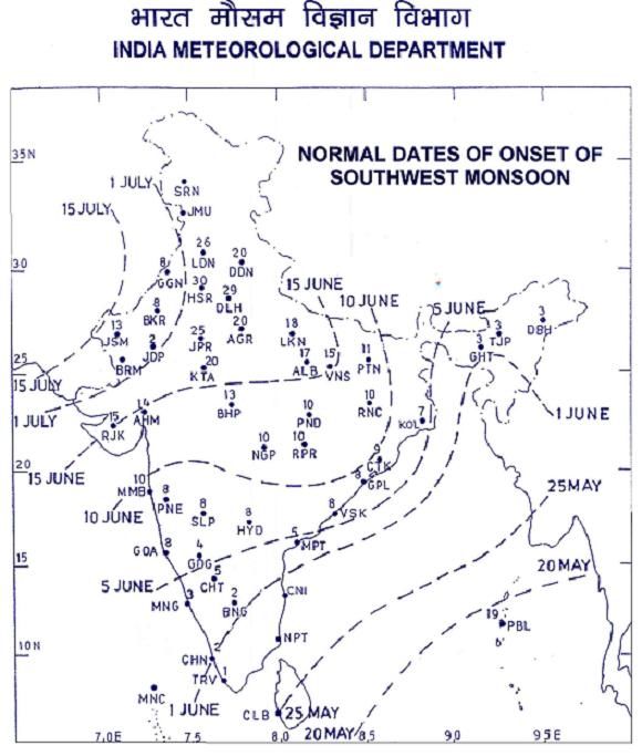
Growing Seasons
• Now explore differential timing of heat shocks
within a calendar year.
• Exploit stark beginning of the agricultural
growing/planting season in India, which is
oriented around the sudden arrival of
(Southwest) monsoon rains in June.
• Studied in detail in AP region by Gine, Townsend
and Vickery (2007).
• Therefore define:
• ‘Growing season’: period between ‘normal’
monsoon arrival (in a district) and December 31st.
• ‘Non-growing season’: three-month period before
‘normal’ monsoon arrival (in a district).‘Normal’ Monsoon Onset From website of Indian Meteorological Department; we map our districts to this.
GS vs NGS Rural only
GS, with Lagged Effects Rural only
GS vs NGS, with Lagged Effects Rural only
GS vs NGS, with Lagged Effects Urban only
GS vs NGS, with Lagged Effects Rural and Urban
Outline of Talk
  Background
     Weather and Human Health
     Simple Theoretical Framework
  Data and Empirical Strategy
  Results:
     Weather and Death
     Weather and Income
  Implications of Climate Change
ConclusionTemperature and Productivity: Rural
Rural Productivity: Real aggregate agricultural output per acre
0.010
0.005
0.000
-0.005
-0.010
Estimated Impact of a Day in 15 Temperature (C) Bins on Log Agricultural Total Product
(Sum Weighted by Average Crop Price), Relative to a Day in the 22° - 24°C Bin
-2 std err coefficient +2 std errWeather and Productivity: R vs U
Rural: real agricultural output per acre;
Urban: (state-level) registered manufacturing output
Rural Urban
Dependent variable: log (productivity)
(1) (2)
Temperature (degree‐days over 32C) ÷ 10 ‐0.0100 ‐0.0000
(0.0035)*** (0.0055)
Rainfall in lower tercile ‐0.0915 ‐0.0435
(0.0097)*** (0.0327)
Rainfall in upper tercile 0.0036 ‐0.0595
(0.0063) (0.0414)
Number of observations 8,604 512
R‐squared 0.87 0.99
Notes: Regressions include district fixed effects, year fixed effects and climatological region‐specific quadratic time
trends. Column (1) regression weighted by average cultivated area; column (2) regression weighted by state urban
population. Standard errors clustered by district.Weather and Productivity: GS vs NGS
Rural only. Real agricultural output per acre
Dependent variable: log (productivity) (1) (2)
GROWING SEASON:
Temperature (degree‐days over 32C) ÷ 10 ‐0.0090 ‐0.0089
(0.0031)*** (0.0031)***
NON‐GROWING SEASON:
Temperature (degree‐days over 32C) ÷ 10 0.0015
(0.0022)
Number of observations 8,604 8,604
R‐squared 0.87 0.87
Notes: Regressions control for rainfall terciles and include district fixed effects, year fixed effects and climatological
region‐specific quadratic time trends. Regressions weighted by average cultivated area. Standard errors clustered
by district.Temperature and Nominal Wages: Rural
Rural Wage: District-level agricultural wage
0.010
0.005
0.000
-0.005
-0.010
Estimated Impact of a Day in 15 Temperature (C) Bins on Log Real Agricultural Wage,
Relative to a Day in the 22° - 24°C Bin
-2 std err coefficient +2 std errTemperature and Nominal Wages: Urban
Urban Wage: State-level earnings per worker in manufacturing sector
0.030
0.020
0.010
0.000
-0.010
-0.020
-0.030
Estimated Impact of a Day in 15 Temperature (C) Bins on Log Manufacturing Wage,
Relative to a Day in the 22° - 24°C Bin
-2 std err coefficient +2 std errWeather and Nominal Wages: R vs U
Rural: Agricultural wages;
Urban: State-level manufacturing earnings per worker
Rural Urban
Dependent variable: log (nominal wage)
(1) (2)
Temperature (degree‐days over 32C) ÷ 10 ‐0.0045 0.0065
(0.0015)*** (0.0057)
Rainfall in lower tercile ‐0.0167 ‐0.0223
(0.0066)** (0.0647)
Rainfall in upper tercile 0.0050 ‐0.0105
(0 0069)
(0.0069) (0 0746)
(0.0746)
Number of observations 7,994 482
R‐squared 0.95 0.96
Notes: Regressions include district fixed effects, year fixed effects and climatological region‐specific quadratic time
trends. Column (1) regression weighted by rural district population; column (2) regression weighted by state urban
population. Standard errors clustered by district.Weather and Nominal Wages: GS vs NGS
Rural only. Nominal agricultural wage
Dependent variable: log (nominal wage) (1) (2)
GROWING SEASON:
Temperature (degree‐days over 32C) ÷ 10 ‐0.0041 ‐0.0043
(0.0015)** (0.0015)**
NON‐GROWING SEASON:
Temperature (degree‐days over 32C) ÷ 10 0.0014
(0.0014)
Number of observations 7,994 7,994
R‐squared 0.95 0.95
Notes: Regressions control for rainfall terciles and include district fixed effects, year fixed effects and climatological
region‐specific quadratic time trends. Regressions weighted by rural population. Standard errors clustered by
district.Temperature and Prices: Rural
Rural Prices: Price index of agricultural prices
0.010
0.005
0.000
-0.005
-0.010
Estimated Impact of a Day in 15 T emperature (C) Bins on Log Agricultural Prices
(Sum Weighted by Average Crop Production), R elative to a D ay in the 22° - 24°C Bin
-2 std err coefficient +2 std errWeather and Prices: R vs U
Rural: Agricultural prices (mostly ‘farm gate’);
Urban: state-level industrial workers’ CPI
Rural Urban
Dependent variable: log (prices)
(1) (2)
Temperature (degree‐days over 32C) ÷ 10 0.0019 0.0014
(0.0007)** (0.0094)
Rainfall in lower tercile 0.0107 0.0108
(0.0029)*** (0.0066)
Rainfall in upper tercile 0.0014 0.0035
(0 0029)
(0.0029) (0 0051)
(0.0051)
Number of observations 7,994 592
R‐squared 0.95 0.99
Notes: Regressions include district fixed effects, year fixed effects and climatological region‐specific quadratic time
trends. Column (1) regression weighted by average cultivated area; column (2) regression weighted by state urban
population. Standard errors clustered by district.Weather and Prices: GS vs NGS
Rural only. Agricultural prices (mostly ‘farm gate’)
Dependent variable: log (prices) (1) (2)
GROWING SEASON:
Temperature (degree‐days over 32C) ÷ 10 0.0019 0.0020
(0.0007)** (0.0008)***
NON‐GROWING SEASON:
Temperature (degree‐days over 32C) ÷ 10 ‐0.0010
(0.0006)
Number of observations 7,994 7,994
R‐squared 0.98 0.98
Notes: Regressions control for rainfall terciles and include district fixed effects, year fixed effects and climatological
region‐specific quadratic time trends. Regressions weighted by average cultivated area. Standard errors clustered
by district.Temperature and Bank Deposits: Rural
Estimated Response Function Between Temperature Exposure and Log Ban
Deposits
Bank Per per
deposits Capita,
capitaRural Areas
in Rural areas
0.020
0.010
0.000
-0.010
-0.020
Estimated Impact of a Day in 15 Temperature (C) Bins on Log Bank Deposits Per Capita,
Relative to a Day in the 22° - 24°C Bin
-2 std impact +2 stdTemperature and Bank Deposits: Urban
Estimated Response Function Between Temperature Exposure and Log Ban
Deposits
Bank Per per
deposits Capita,
capitaUrban Areas
in Urban areas
0.020
0.010
0.000
-0.010
-0.020
Estimated Impact of a Day in 15 Temperature (C) Bins on Log Bank Deposits Per Capita,
Relative to a Day in the 22° - 24°C Bin
-2 std impact +2 stdOutline of Talk
Background
Weather and Human Health
Simple Theoretical Framework
Data and Empirical Strategy
Results:
Weather and Death
Weather and Income
Implications of Climate Change
ConclusionImplications of Climate Change I
• We have documented a large reduced-form
impact of both temperature and rainfall
extremes on mortality in India from 1956-2000
• Looking into the future: As India’s climate
changes throughout the 21st Century, what are
the implications for mortality?
• Clearly one has to be very skeptical of the use of
reduced-form estimates based on the past to
predict the future.
• But it is unclear what the alternative is.
• Under most scenarios, our estimates (based on
short-lived shocks) will place an upper-bound on
the effects of a long-run change.Implications of Climate Change II
• Climatological models predict ∆Td (and
∆RAINd , though these are more controversial)
• We use our earlier estimates of the mortality
consequences of weather variation to estimate
the mortality consequences of predicted ∆Td :
X 3
X
∆Y
dd = θbj ∆Tdj + δbk ∆1 {RAINd in tercile k}
j k=1
• Report pop-weighted average of these
district-level impacts.Implications of Climate Change III
• Feed in 2 standard C.C. models:
1. Hadley Centre’s 3 A1F1 (corrected) model and
NCAR’s CCSM 3 A2 model
• Both are ‘business as usual’ scenarios (no CO2
mitigation)
• Both do not include ‘catastrophic scenarios’
(Himalayan glaciers melt, monsoon terminates, sea
level rises, more cyclones)
• Details:
• Models simulate full daily time path of temp. and
rain from 1990-2099
• Different time paths for each district in India
• Define ∆Td ≡ Td2070−2099 − Td1957−2001 etc
• Compute ∆Y dd for each district d and take
population-weighted averagePredicted Change in Temp. Distribution
60
40
20
0
-20
-40
Predicted Change in Distribution of Daily Mean Temperatures (C),
Change in Days Per Year in Each Interval
CCSM 3 A2 Hadley 3 A1FI, CorrectedClimate Change and Mortality
dd = P θbj ∆T j + P3 δbk ∆1 {RAINd in tercile k}
Percentage impacts: ∆Y j d k=1
in 2070-2099 (on average)
Temperature
Impact of Change in Days with Total
and
Temperature: Temperature
Precipitation
Impact
< 16 C 16 C‐32 C > 32 C Impacts
(1a) (1b) (1c) (2) (3)
Based on Hadley 3, A1F1
Pooled ‐0.010 ‐0.139 0.659 0.510 0.462
(0.030) (0.045) (0.126) (0.125) (0.142)
Rural Areas ‐0.030 ‐0.164 0.853 0.658 0.617
(0.039) (0.055) (0.153) (0.126) (0.173)
Urban Areas 0.036 0.013 0.090 0.112 0.116
(0.033) (0.058) (0.105) (0.101) (0.116)
Based on CCSM3, A2
Pooled ‐0.010 0.039 0.145 0.176 0.116
(0.013) (0.042) (0.028) (0.061) (0.084)
Rural Areas ‐0.015 0.071 0.189 0.245 0.207
(0.016) (0.049) (0.035) (0.074) (0.099)
Urban Areas 0.009 0.016 0.028 0.052 ‐0.078
(0.013) (0.042) (0.022) (0.054) (0.092)Climate Change and Mortality
dd = P θbj ∆T j + P3 δbk ∆1 {RAINd in tercile k}
Percentage impacts: ∆Y j d k=1
All India
Temperature
Impact of Change in Days with Total
and
Temperature: Temperature
Precipitation
Impact
< 16 C 16 C‐32 C > 32 C Impacts
(1a) (1b) (1c) (2) (3)
Based on Hadley 3, A1F1
2010‐2039 ‐0.009 0.027 0.057 0.075 0.037
(0.014) (0.026) (0.012) (0.039) (0.054)
2040‐2069 ‐0.011 ‐0.013 0.270 0.246 0.205
(0.025) (0.028) (0.050) (0.069) (0.086)
2070‐2099 ‐0.010 ‐0.139 0.659 0.510 0.462
(0.030) (0.045) (0.126) (0.125) (0.142)
Based on CCSM3, A2
2010‐2039 ‐0.006 0.082 ‐0.073 0.003 ‐0.054
(0.010) (0.016) (0.015) (0.018) (0.041)
2040‐2069 ‐0.008 0.097 0.002 0.091 0.031
(0.006) (0.023) (0.005) (0.023) (0.050)
2070‐2099 ‐0.008 0.039 0.145 0.176 0.116
(0.013) (0.042) (0.028) (0.061) (0.084)Outline of Talk
Background
Weather and Human Health
Simple Theoretical Framework
Data and Empirical Strategy
Results:
Weather and Death
Weather and Income
Implications of Climate Change
ConclusionSummary: Aim to Make 3 Contributions
1. Document new facts about the role that
temperature extremes play in the mortality
risks faced by LDC residents.
• One SD more degree-days (over 32 C) leads to 9
% higher crude death rate. (20 × US effect.)
2. Understand the plausibility of various
mechanisms that could explain these effects.
• Cluster of findings (rural not urban, GS not NGS,
mirror effects in rural incomes) consistent with
these effects working through agricultural income.
3. Use these estimates to inform estimates of
health costs of climate change scenarios.
• No-adaptation (upper-bound) costs: annual
mortality rate to rise by 10-50%.Summary: Implications
• Smoothing of marginal utility in rural India
seems far from complete.
• Aggregate (between-village) income/health shocks
are not being insured in the way that idiosyncratic
(within-village) shocks are (eg Townsend (1994)).
• Weather-dependent income transfers are likely
to save lives cheaply.
• Temperature extremes seem to matter a great
deal already for rural incomes and health
status.
• And this will only get worse (or costly adaptations
will be incurred) if temperatures rise in the future.You can also read


