WeatherBench Probability: A benchmark dataset for probabilistic medium-range weather forecasting along with deep learning baseline models
←
→
Page content transcription
If your browser does not render page correctly, please read the page content below
WeatherBench Probability: A benchmark dataset for
                                                 probabilistic medium-range weather forecasting
                                                     along with deep learning baseline models
arXiv:2205.00865v1 [physics.ao-ph] 2 May 2022

                                                                        Sagar Garg                                    Stephan Rasp
                                                          Technical University of Munich, Germany                     ClimateAi, Inc
                                                                                                                 raspstephan@gmail.com

                                                                                          Nils Thuerey
                                                                             Technical University of Munich, Germany

                                                                                             Abstract

                                                         WeatherBench is a benchmark dataset for medium-range weather forecasting
                                                         of geopotential, temperature and precipitation, consisting of preprocessed data,
                                                         predefined evaluation metrics and a number of baseline models. WeatherBench
                                                         Probability extends this to probabilistic forecasting by adding a set of established
                                                         probabilistic verification metrics (continuous ranked probability score, spread-skill
                                                         ratio and rank histograms) and a state-of-the-art operational baseline using the
                                                         ECWMF IFS ensemble forecast. In addition, we test three different probabilistic
                                                         machine learning methods—Monte Carlo dropout, parametric prediction and cate-
                                                         gorical prediction, in which the probability distribution is discretized. We find that
                                                         plain Monte Carlo dropout severely underestimates uncertainty. The parametric
                                                         and categorical models both produce fairly reliable forecasts of similar quality. The
                                                         parametric models have fewer degrees of freedom while the categorical model is
                                                         more flexible when it comes to predicting non-Gaussian distributions. None of the
                                                         models are able to match the skill of the operational IFS model. We hope that this
                                                         benchmark will enable other researchers to evaluate their probabilistic approaches.

                                                1   Introduction

                                                WeatherBench [Rasp et al., 2020] introduced a benchmark dataset for medium-range, data-driven
                                                weather forecasting, focused on 3 and 5 day predictions of global geopotential, temperature and
                                                precipitation fields. The three core components of WeatherBench are 1) a preprocessed training
                                                and validation dataset hosted in a convenient format on a public server, 2) a set of precisely defined
                                                evaluation metrics and 3) a set of baselines, ranging from simple ones such as climatologies and
                                                persistence to dynamical models run at different resolutions and simple machine learning models.
                                                The idea behind WeatherBench is to provide a framework in which to evaluate progress in data-driven
                                                weather forecasting. Since its publication, WeatherBench has been used in several papers. Weyn
                                                et al. [2020] built a convolutional neural network (CNN) trained using a cubed-sphere coordinate
                                                transformation. They then extended this approach for subseasonal prediction [Weyn et al., 2021].
                                                Rasp and Thuerey [2021] used a deep Resnet architecture pretrained on climate model simulations
                                                that achieves comparable skill to dynamical baselines at similar resolutions. Gneiting and Walz
                                                [2019] used the WeatherBench dataset to compare different evaluation metrics. Keisler [2022] trained
                                                a graph neural network and achieved impressive skill on metrics very similar to those suggested in
                                                WeatherBench.

                                                Preprint. Under review.
One short-coming of the original WeatherBench benchmark is that it exclusively focuses on determin-
istic prediction. However, in medium-range weather forecasting is was long ago recognized that the
inherent unpredictability of the atmosphere necessitates a probabilistic approach [Bauer et al., 2015].
For this reason, virtually all operational weather forecasting centers run ensemble forecasts, where
each ensemble member represents one realistic potential future outcome. Here we aim to extend
WeatherBench by adding a probabilistic dimension to the verification metrics and baselines. Building
on this we then train a range of probabilistic neural networks.
There is some previous work in building probabilistic data-driven methods. Scher and Messori
[2020] tested several methods to create a data-driven ensemble forecast: random initial condition
perturbations, singular vector initial condition perturbations and different random seeds for the neural
networks. The latter results in the best probabilistic scores. Clare et al. [2021] explored dropout
ensembles, similar to this work. We will contrast our results to theirs below.
We begin by briefly summarizing the original WeatherBench data and describing the new evaluation
metrics and baselines in Section 2. Then, in Section 3 we review relevant literature in probabilistic
machine learning before describing the three methods we will use. This is followed by the results of
our methods in Section 4, which we discuss further in Section 5, before summarizing our findings in
Section 6.
2 Data, Evaluation and Baselines
2.1 Data
Here we will provide a brief summary of the WeatherBench dataset. For a detailed description
refer to Rasp et al. [2020]. The latest version of the data is available at https://github.com/
pangeo-data/WeatherBench. WeatherBench contains regridded ERA5 [Hersbach et al., 2020]
data from 1979 to 2018 at hourly resolution with 2017 and 2018 set aside for evaluation. Here we use
the coarsest horizontal resolution, 5.625◦ (32 × 64 grid points), at 7 vertical levels (50, 250, 500,
600, 700, 850, and 925 hPa).
As a probabilistic baseline we use the 50-member operational ECMWF IFS ensemble, archived in
the THORPEX Interactive Grand Global Ensemble (TIGGE) archive [Bougeault et al., 2010]. The
target variables 500 hPa geopotential (Z500), 850 hPa temperature (T850), 2 m temperature (T2M)
and 6h accumulated precipitation (PR) for 2017 and 2018 regridded to match WeatherBench are now
also available at Rasp [2022].
2.2 Evaluation
For evaluating the probabilistic forecasts, we chose several well-established metrics. First, we
evaluate the deterministic skill of the ensemble mean using the root mean squared error (RMSE)
defined as
v
N N
lat NX
u
1 forecasts
X u
1 X lon
L(j)(f¯i,j,k − ti,j,k )2
u
RMSE = t (1)
Nforecasts i
Nlat Nlon j
k
where f¯ is the ensemble mean forecast and t is the ERA5 truth. L(j) is the latitude weighting factor
for the latitude at the jth latitude index:
cos(lat(j))
L(j) = PNlat (2)
1
N j cos(lat(j))
lat
As a first-order measure of the reliability of the ensemble, we look at the spread-skill ratio
(Spread/RMSE), where Spread defined as
v
N N
lat NX
u
1 forecasts
X u
u 1 X lon
Spread = t L(j)var(fj,k ) (3)
Nforecasts i
Nlat Nlon j
k
2where var(fj,k ) is the variance in the ensemble dimension. A perfectly reliable ensemble should have
a spread-skill ratio of 1. Smaller values indicate underdispersion (i.e. the probabilistic forecast is
overconfident in its forecasts), larger values overdispersion [Fortin et al., 2014].
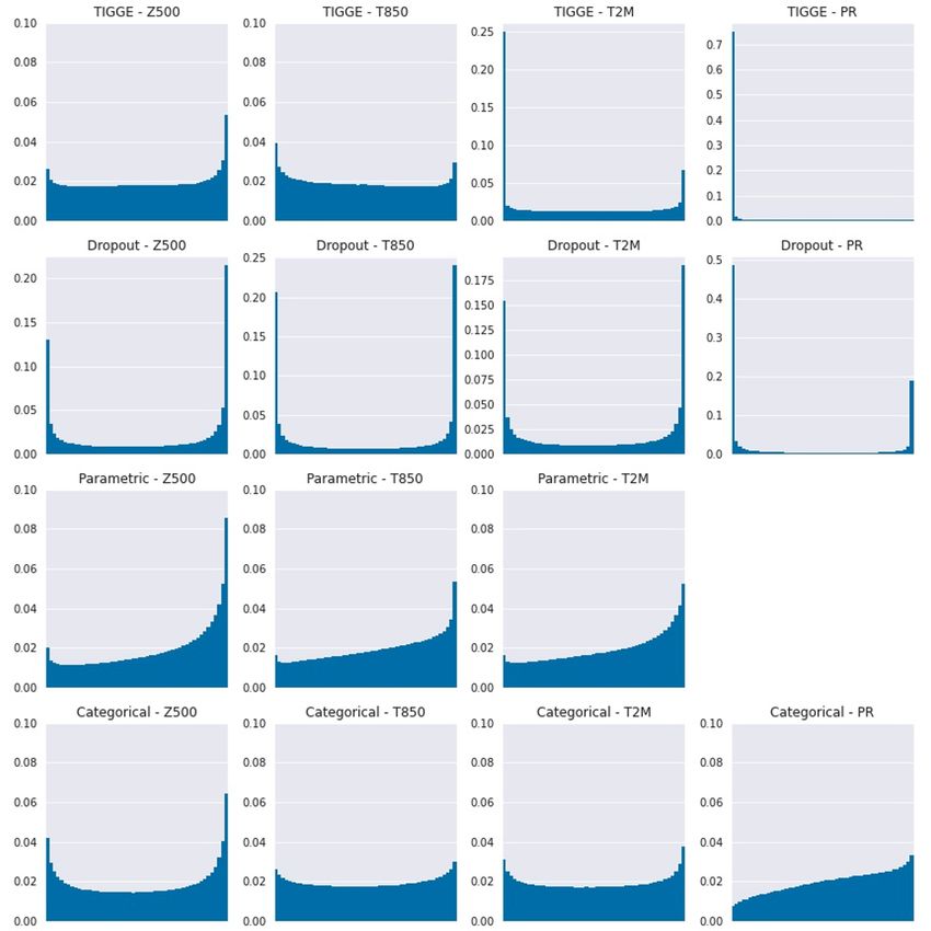
As a more detailed visual evaluation of reliability we use rank histograms, described in detail in Wilks
[2006](p. 316). A perfect rank histogram is uniform, while a U-shape indicates underdispersion and
a reverse U-shape overdispersion.
Finally, calibration and sharpness of the ensemble together is evaluated using the continuous ranked
probability score (CRPS) Wilks [2006](p. 302), defined as:
Z ∞
CRPS = [F (f ) − 1(t ≤ z)]2 dz, (4)
−∞
where F denotes the CDF of the forecast distribution and 1(t ≤ z) is an indicator function that is
1 if t ≤ z and 0 otherwise. In the case of a deterministic forecast the CRPS reduces to the mean
absolute error. For computing the CRPS for ensemble forecasts, we use the implementation in the
xskillscore1 Python package.
3 Probabilistic neural networks
We explore three different methods to create probabilistic predictions using neural networks. The
basic network architecture of all networks is a deep Resnet, which mirrors that of Rasp and Thuerey
[2021] with only the final layer changed. The input variables are geopotential, temperature, zonal
and meridional wind and specific humidity at seven vertical levels (50, 250, 500, 600, 700, 850 and
925hPa), 2-meter temperature, 6-hourly accumulated precipitation, the top-of-atmosphere incoming
solar radiation, all at the current time step t, t − 6h and t − 12h, and, finally three constant fields:
the land-sea mask, orography and the latitude at each grid point. All variables, levels and time
steps are stacked to create a 114 channel input. All features are normalized (x ← x−mean std ),
except precipitation where mean = 0 to keep values positive. Precipitation is also log-transformed
(PR ← log(PR + ) − log()), where = 0.001. For evaluation the transformation is reversed again.
All models were trained using ERA5 data from 1979 to 2015, with 2016 used for validation and
2017/18 for testing. Predictions are made for a lead-time of 3 days.2 The training procedure is the
same as in Rasp and Thuerey [2021]. No pretraining with climate models was used for any of the
experiments in this paper.
3.1 Monte-Carlo Dropout (MC Dropout)
Dropout [Srivastava et al., 2014] was introduced as a simple way of combating overfitting in neural
networks. Typically, dropout is only applied during training but then turned off during inference. In
fact, our base architecture described above uses dropout with a rate of 0.1. However, it is also possible
to use dropout during inference to obtain a stochastic prediction [Gal and Ghahramani, 2015]. Here
we train our model with different dropout rates, 0, 0.1, 0.2 and 0.5, and create 50 random realizations
for the test dataset to match the 50-member IFS ensemble.
3.2 Parametric prediction
Another way to create a probabilistic forecast using neural networks is to directly predict the
parameters of a distribution. This is a common technique in ensemble post-processing. Here we
follow the methodology of Rasp and Lerch [2018]. The first step is to prescribe a distribution for
the target variables. For Z500, T850 and T2M we use a Gaussian distribution parameterized by its
mean µ and variance σ. This means that instead of a single output channel, the network now has
two channels for µ and σ. To optimize for the distributional parameters we chose the CRPS as a
probabilistic loss function. For a Gaussian distribution, there exists a closed-form, differentiable
1
https://xskillscore.readthedocs.io
2
Ideally we would have also trained models for 5 days lead time and continuous models. However, because
the first two authors moved on to different positions shortly after the initial work was finished, this was not
possible. We would expect qualitatively similar results for other lead times.
3Table 1: RMSE, Spread-skill ratio and CRPS for different methods for 3 day forecasts.
RMSE of ensemble mean Spread-Skill Ratio CRPS
Z500 (m2 s−2 ) T850 (K) T2M (K) TP (mm) Z500 T850 T2M TP Z500 (m2 s−2 ) T850 (K) T2M (K) TP (mm)
MC Dropout
312.96 1.80 1.52 2.2 0.40 0.34 0.39 0.13 155.70 1.03 0.77 0.57
(Dr=0.1)
Parametric 315.30 1.82 1.55 - 0.87 0.92 0.95 - 142.67 0.90 0.70 -
Categorical 327.48 1.80 1.49 2.2 0.91 0.94 0.98 1.24 142.59 0.87 0.65 0.47
Tigge (3/5 days) 145/297 1.20/1.73 1.26/1.57 2.02/2.15 1.05/1.00 0.93/0.96 0.69/0.80 0.84/0.85 65.6/127 0.60/0.83 0.58/0.70 0.41/0.47
Determinstic 313.70 1.79 1.53 2.2 - - - - 194.90 1.24 0.96 0.65
Clare et al. [2021] 375/627 2.11/2.91 211/1500 1.22 / 1.69
solution of the CRPS:
y−µ y−µ y−µ 1
CRP S (Fµ,σ , y) = σ 2Φ − 1 + 2ϕ −√ (5)
σ σ σ π
For precipitation, a Gaussian distribution would be a poor fit because precipitation tends to be very
skewed and is censored at zero. Several distributions have been proposed in literature such as a
left-censored generalized extreme value distribution [Scheuerer, 2014a]. We struggled to implement
these for neural network training. The closed-forms of these distributions are quite complicated with
limited valid ranges for some parameters. Unfortunately, we did not end up figuring out how to
achieve a stable training using these distributions. We will discuss this in Section 5.
For evaluating the parametric forecasts we computed the CRPS and the spread-skill ratio directly
from the predicted parametric distributions but created a randomly sampled 50-member ensemble for
computing the rank histogram to match the other methods.
3.3 Categorical prediction
Finally, we test a non-parametric, probabilistic method based on discretized bins. This has recently
been used by Sønderby et al. [2020] and Espeholt et al. [2021] for precipitation nowcasting. The idea
is to divide the value range to be predicted into discrete bins and predict the probability for each of
these bins. The problem is then simply a multi-class classification problem. The number of channels
in the last layer are changed to match the number of bins, followed by a softmax layer. The targets
are one-hot encoded, with a one indicating the correct bin and zeros otherwise. As a loss function we
use the standard categorical cross-entropy, also called log-loss
There are some subtleties in how to construct the bins. Generally, there is a trade-off between the
bin width, which can be thought of as the probabilistic resolution, and the number of bins. Higher
resolution will lead to finer probability distributions but will also make training harder. Further, the
residual blocks of the core architecture have 128 channels which sets an upper limit to the number of
channels. However, taking temperature prediction as an example, temperature values can fluctuate
by around 100C from the poles to the deserts, which means that the bins would be rather large. For
this reason, for geopotential and temperature, we predict the change in time (Xt=3d − Xt=0 ; after
normalization) rather than the absolute values. These differences will have a much smaller spread.
Before evaluation, we then simply add the difference.
Note that we train our model separately for each variable, unlike in the other experiments where Z,
T, T2M are trained together and precipitation trained separately. Empirically, this has given better
results compared to training all variables together. For Z, T and T2M, we use 50 bins ranging from
-1.5 to 1.5. For precipitation, we use 50 bins from 0 to 8 (after the log-transform).
4 Results
The results for the different verification metrics are shown in Table 1 and Fig. 1. For MC dropout we
also tested the sensitivity to the dropout rate, shown in Fig. 2 (only Z500 is shown; other variables
behave qualitatively similarly). The ensemble mean RMSE and the CRPS is lowest for a dropout rate
of 0.1. The spread-skill ratio shows that the dropout ensemble is severely underdispersive with the
spread being less than half of what it should be. These results are consistent with Clare et al. [2021].
Increasing the dropout rate beyond 0.1 has a slight positive effect on the spread-skill ratio but this
comes at the cost of severely decreasing skill measured by the ensemble mean RMSE and CRPS. This
will be further discussed in Section 5. For now, we use a dropout rate of 0.1 for all further evaluation.
4Figure 1: (top) Ensemble mean RMSE for TIGGE baseline and different data-driven methods.
(bottom) Same for CRPS.
5Embsemble-mean RMSE CRPS Spread-skill ratio
380 210 0.4
Z500 RMSE [m2 s 2]
Z500 CRPS [m2 s 2]
200
0.3
Spread / Skill
360
190
180 0.2
340
170 0.1
320 160
0.0
0.0 0.1 0.2 0.5 0.0 0.1 0.2 0.5 0.0 0.1 0.2 0.5
Dropout rate Dropout rate Dropout rate
Figure 2: RMSE, CRPS and spread-skill ratio for different dropout rates for Z500.
The ensemble mean RMSE is reasonably similar between all deep learning methods with slight
fluctuations between the variables. We also added the RMSE of the deterministic deep learning model
without pretraining described in Rasp and Thuerey [2021] as well as the scores reported in Clare et al.
[2021]. The operational TIGGE ensemble outperforms the data-driven methods quite significantly.
The only exception is precipitation, but, as already discussed in Rasp and Thuerey [2021], the RMSE
is not a particularly fitting metric to evaluate a highly intermittent and skewed field like precipitation.
The spread-skill ratio shows that MC dropout is severely underdispersive for all variables. The para-
metric and categorical networks have similar ratios just under one for geopotential and temperature,
while the ratio is above one for categorical precipitation. TIGGE has ratios very close to one for Z500
and T850 but is somewhat underdispersive for T2M. It is important to remember here though that the
TIGGE results are not post-processed, which would likely improve calibration.
Further insight into calibration and reliability can be gained from looking at the rank histograms
in Fig. 3. Here, we see a very strong U-shape for MC dropout. TIGGE only has a slight U-shape
for Z500 and T850 but strong peaks on the left-hand side for T2M and PR. For T2M, this hints at a
bias issue but would require further investigation. The peak for PR could be a manifestation of the
well-known drizzle bias. The parametric predictions are skewed which is a sign of a high-bias. We
did not further investigate the cause for this. The categorical predictions do not have a bias and are
only moderately U-shaped, suggesting good calibration.
The CRPS evaluates both calibration and sharpness. Again we see similar scores for the parametric
and categorical networks, with slightly better results for categorical. MC dropout is worse on CRPS,
a consequence of its underdispersion. Further, we see that the deterministic forecast (for which
the CRPS is simply the MAE) naturally scores worse since it does not provide any probabilistic
information. Again, TIGGE has significantly better CRPS scores compared to the data driven
methods.
5 Discussion
5.1 Verification caveats
There are several aspects to consider in the above verification. First, the verification is done at a very
coarse grid, 5.625 degrees. The operational IFS ensemble forecast runs at a resolution of around 13
km. The required regridding could potentially add a source of error, which might partly account for
the initial error at t = 0h of the operational ensemble. However, another cause of initial error is the
fact that the operational forecasts are started from different initial conditions, the operational analysis
as opposed to the ERA5 reanalysis. For a fair comparison of pure forecasting skill, each method
should be compared against its own analysis, starting from zero error at t = 0h.
For precipitation, the verification metrics used, RMSE and CRPS, are poor choices as they suffer
heavily from the double penalty problem. In the original WeatherBench paper and here, we still
decided to include the metrics but urge everyone to interpret these results with the appropriate caution.
5.2 Parametric versus categorical prediction
Both, parametric and categorical forecasts performed well in this study, with similar verification
scores. They also both have been used successfully in previous research, even if parametric methods
6Figure 3: Rank histograms for different variables and methods. All rank histograms have 51 bins.
have a much longer history, especially in post-processing. Parametric approaches have the advantage
of simplicity. Only a few (usually 2-3) parameters are to be estimated to produce a full distribution.
For parameters where the underlying distribution is thought to be well known, e.g. temperature
and geopotential, a parametric approach is a great choice. However, for more unusually distributed
variables, e.g. precipitation, problems can arise. First, often the "true" distribution is not know which
requires assumptions to be made. If those assumptions are not true, an artificial error is introduced.
Second, more complex distribution functions and their derivatives required for gradient descent
optimization can be difficult to implement. In the case of precipitation, we attempted to implement
a censored extreme value distribution described in Scheuerer [2014b]. However, we encountered
exploding gradients during optimization, likely a result of the limited valid ranges of some of the
distributional parameters. One could likely fix this by adding constraints on the parameter values
and tinkering with the implementation of the loss. However, it shows some of the difficulty with the
parametric approach.
The categorical approach, on the other hand, requires no assumptions on the distribution. In theory,
any distribution can be learned. This is potentially a big advantage of this method, especially for
more complex distributions. The trade-off is that instead of learning 2-3 values, now >100 values
have to be estimated, which can be problematic for small sample sizes. In fact, we have observed that
initially the estimated "distributions" are not smooth and only become so after training. Further, one
introduces a probabilistic resolution, i.e. the bin width. As described in the Methods, this required
7a reframing of the problem for geopotential and temperature to predict the change rather than the
absolute value. Nevertheless, the categorical approach, given enough samples, turns out to work very
well empirically and is easy to implement.
5.3 Spatially and temporally correlated forecasts
A final topic to discuss is spatial correlation in the forecast fields. The parametric and categorical
methods predict separate distributions at each grid point and at each point in time. While this is fine
for some applications, others also require knowledge about spatial and temporal patterns. For flood
forecasting, for example, one is not simply interested in the distribution of rain at a single location in 5
days time but rather in the distribution of cumulative rain in the entire catchment area. For rain, which
can have very different characteristics, e.g. convective versus stratiform, adding the distributions in
space and time will not lead to the correct answer. Further, visual inspection of weather maps is still
a very common use case for decision makers. With point-wise distribution methods, it is impossible
to create "realistic" weather maps. Monte-Carlo dropout produces an ensemble of spatially coherent
outputs but produces less reliable results compared to the other methods.
To solve this issue, generative methods could be an option. Generative adversarial networks (GANs)
[Goodfellow et al., 2014] are one way of producing realistic weather output. Recently this has been
used for precipitation nowcasting [Ravuri et al., 2021] and downscaling [Price and Rasp, 2022, Harris
et al., 2022]. While GANs are, in principal, a well-suited method to produce coherent output, in
practice they can be hard to train and empirically don’t always produce the correct distribution.
6 Conclusion
Here we introduced WeatherBench Probability, a probabilistic extension to the WeatherBench bench-
mark dataset. We added commonly used probabilistic verification metrics along with an operational
numerical weather prediction baseline. Further, we trained three different sets of deep learning
models to produce probabilistic predictions for 3 days ahead, Monte-Carlo dropout, parametric and
categorical networks. Our version of Monte-Carlo dropout produced severely underdispersive results.
The other two methods produced similarly good results across all scores, with trade-offs between the
two discussed in Section 5.
We hope that this paper complements the WeatherBench dataset and enables fast and easy comparison
between different data-driven forecasting methods. In the last year or two, a number of promising
approaches have been proposed and others are in development which makes for an exciting future for
this research field.
References
Stephan Rasp, Peter D. Dueben, Sebastian Scher, Jonathan A. Weyn, Soukayna Mouatadid, and Nils
Thuerey. WeatherBench: A Benchmark Data Set for Data-Driven Weather Forecasting. Journal
of Advances in Modeling Earth Systems, 12(11), 11 2020. ISSN 1942-2466. doi: 10.1029/
2020MS002203. URL https://onlinelibrary.wiley.com/doi/10.1029/2020MS002203.
Jonathan A. Weyn, Dale R. Durran, and Rich Caruana. Improving Data-Driven Global Weather
Prediction Using Deep Convolutional Neural Networks on a Cubed Sphere. Journal of Advances
in Modeling Earth Systems, 12(9), 9 2020. ISSN 1942-2466. doi: 10.1029/2020MS002109. URL
https://onlinelibrary.wiley.com/doi/10.1029/2020MS002109.
Jonathan A. Weyn, Dale R. Durran, Rich Caruana, and Nathaniel Cresswell-Clay.
Sub-Seasonal Forecasting With a Large Ensemble of Deep-Learning Weather
Prediction Models. Journal of Advances in Modeling Earth Systems, 13(7):
e2021MS002502, 7 2021. ISSN 1942-2466. doi: 10.1029/2021MS002502. URL
https://onlinelibrary.wiley.com/doi/full/10.1029/2021MS002502https:
//onlinelibrary.wiley.com/doi/abs/10.1029/2021MS002502https://agupubs.
onlinelibrary.wiley.com/doi/10.1029/2021MS002502.
Stephan Rasp and Nils Thuerey. Data-Driven Medium-Range Weather Prediction With a Resnet
Pretrained on Climate Simulations: A New Model for WeatherBench. Journal of Advances
in Modeling Earth Systems, 13(2):e2020MS002405, 2 2021. ISSN 19422466. doi: 10.1029/
2020MS002405. URL https://github.com/pangeo-data/WeatherBench.
8Tilmann Gneiting and Eva-Maria Walz. Receiver operating characteristic (ROC) movies, universal
ROC (UROC) curves, and coefficient of predictive ability (CPA). arXiv, 11 2019. URL http:
//arxiv.org/abs/1912.01956.
Ryan Keisler. Forecasting Global Weather with Graph Neural Networks. 2 2022. doi: 10.48550/
arxiv.2202.07575. URL https://arxiv.org/abs/2202.07575v1.
Peter Bauer, Alan Thorpe, and Gilbert Brunet. The quiet revolution of numerical weather pre-
diction. Nature, 525(7567):47–55, 9 2015. ISSN 0028-0836. doi: 10.1038/nature14956.
URL http://www.nature.com.emedien.ub.uni-muenchen.de/nature/journal/v525/
n7567/full/nature14956.html.
Sebastian Scher and Gabriele Messori. Ensemble neural network forecasts with singular value
decomposition. 2 2020. URL https://arxiv.org/abs/2002.05398.
Mariana Clare, Omar Jamil, and Cyril Morcrette. A computationally efficient neural network for
predicting weather forecast probabilities. 3 2021. URL http://arxiv.org/abs/2103.14430.
Hans Hersbach, Bill Bell, Paul Berrisford, Shoji Hirahara, András Horányi, Joaquín Muñoz-Sabater,
Julien Nicolas, Carole Peubey, Raluca Radu, Dinand Schepers, Adrian Simmons, Cornel Soci,
Saleh Abdalla, Xavier Abellan, Gianpaolo Balsamo, Peter Bechtold, Gionata Biavati, Jean Bidlot,
Massimo Bonavita, Giovanna Chiara, Per Dahlgren, Dick Dee, Michail Diamantakis, Rossana
Dragani, Johannes Flemming, Richard Forbes, Manuel Fuentes, Alan Geer, Leo Haimberger, Sean
Healy, Robin J. Hogan, Elías Hólm, Marta Janisková, Sarah Keeley, Patrick Laloyaux, Philippe
Lopez, Cristina Lupu, Gabor Radnoti, Patricia Rosnay, Iryna Rozum, Freja Vamborg, Sebastien
Villaume, and Jean-Noël Thépaut. The ERA5 Global Reanalysis. Quarterly Journal of the Royal
Meteorological Society, page qj.3803, 5 2020. ISSN 0035-9009. doi: 10.1002/qj.3803. URL
https://onlinelibrary.wiley.com/doi/abs/10.1002/qj.3803.
Philippe Bougeault, Zoltan Toth, Craig Bishop, Barbara Brown, David Burridge, De Hui Chen,
Beth Ebert, Manuel Fuentes, Thomas M. Hamill, Ken Mylne, Jean Nicolau, Tiziana Paccagnella,
Young-Youn Park, David Parsons, Baudouin Raoult, Doug Schuster, Pedro Silva Dias, Richard
Swinbank, Yoshiaki Takeuchi, Warren Tennant, Laurence Wilson, and Steve Worley. The THOR-
PEX Interactive Grand Global Ensemble. Bulletin of the American Meteorological Society, 91(8):
1059–1072, 8 2010. doi: 10.1175/2010BAMS2853.1. URL http://journals.ametsoc.org/
doi/10.1175/2010BAMS2853.1.
Stephan Rasp. TIGGE data for WeatherBench Probability. 4 2022. doi: 10.5281/ZENODO.6480846.
URL https://doi.org/10.5281/zenodo.6480846#.YmVG6z5Nf1o.mendeley.
V. Fortin, M. Abaza, F. Anctil, and R. Turcotte. Why Should Ensemble Spread Match the RMSE of
the Ensemble Mean? Journal of Hydrometeorology, 15(4):1708–1713, 8 2014. ISSN 1525-755X.
doi: 10.1175/JHM-D-14-0008.1. URL http://journals.ametsoc.org/doi/abs/10.1175/
JHM-D-14-0008.1.
Daniel S Wilks. Statistical Methods in the Atmospheric Sciences. Elsevier, 2006. ISBN 0127519661.
URL http://cds.cern.ch/record/992087.
Nitish Srivastava, Geoffrey Hinton, Alex Krizhevsky, Ilya Sutskever, and Ruslan Salakhutdi-
nov. Dropout: A Simple Way to Prevent Neural Networks from Overfitting. Journal of
Machine Learning Research, 15:1929–1958, 2014. URL http://www.jmlr.org/papers/
volume15/srivastava14a/srivastava14a.pdf?utm_content=buffer79b43&utm_
medium=social&utm_source=twitter.com&utm_campaign=buffer.
Yarin Gal and Zoubin Ghahramani. Dropout as a Bayesian Approximation: Representing Model
Uncertainty in Deep Learning. 33rd International Conference on Machine Learning, ICML 2016,
3:1651–1660, 6 2015. URL http://arxiv.org/abs/1506.02142.
Stephan Rasp and Sebastian Lerch. Neural Networks for Postprocessing Ensemble Weather Forecasts.
Monthly Weather Review, 146(11):3885–3900, 11 2018. doi: 10.1175/MWR-D-18-0187.1. URL
http://journals.ametsoc.org/doi/10.1175/MWR-D-18-0187.1.
M. Scheuerer. Probabilistic quantitative precipitation forecasting using Ensemble Model Output
Statistics. Quarterly Journal of the Royal Meteorological Society, 140(680):1086–1096, 4 2014a.
ISSN 00359009. doi: 10.1002/qj.2183. URL http://doi.wiley.com/10.1002/qj.2183.
Casper Kaae Sønderby, Lasse Espeholt, Jonathan Heek, Mostafa Dehghani, Avital Oliver, Tim
Salimans, Shreya Agrawal, Jason Hickey, and Nal Kalchbrenner. MetNet: A Neural Weather
Model for Precipitation Forecasting. 3 2020. URL http://arxiv.org/abs/2003.12140.
9Lasse Espeholt, Shreya Agrawal, Casper Sønderby, Manoj Kumar, Jonathan Heek, Carla Bromberg,
Cenk Gazen, Jason Hickey, Aaron Bell, and Nal Kalchbrenner. Skillful Twelve Hour Precipitation
Forecasts using Large Context Neural Networks. 11 2021. doi: 10.48550/arxiv.2111.07470. URL
https://arxiv.org/abs/2111.07470v1.
M. Scheuerer. Probabilistic quantitative precipitation forecasting using Ensemble Model Output
Statistics. Quarterly Journal of the Royal Meteorological Society, 140(680):1086–1096, 4 2014b.
ISSN 00359009. doi: 10.1002/qj.2183. URL http://doi.wiley.com/10.1002/qj.2183.
Ian Goodfellow, Jean Pouget-Abadie, Mehdi Mirza, Bing Xu, David Warde-Farley, Sherjil Ozair,
Aaron Courville, and Yoshua Bengio. Generative adversarial nets. In Advances in neural informa-
tion processing systems, pages 2672–2680, 2014.
Suman Ravuri, Karel Lenc, Matthew Willson, Dmitry Kangin, Remi Lam, Piotr Mirowski, Megan
Fitzsimons, Maria Athanassiadou, Sheleem Kashem, Sam Madge, Rachel Prudden, Amol Mand-
hane, Aidan Clark, Andrew Brock, Karen Simonyan, Raia Hadsell, Niall Robinson, Ellen Clancy,
Alberto Arribas, and Shakir Mohamed. Skillful Precipitation Nowcasting using Deep Generative
Models of Radar. 4 2021. URL https://arxiv.org/abs/2104.00954v1.
Ilan Price and Stephan Rasp. Increasing the accuracy and resolution of precipitation forecasts
using deep generative models. page 2022, 3 2022. doi: 10.48550/arxiv.2203.12297. URL
https://arxiv.org/abs/2203.12297v1.
Lucy Harris, Andrew T. T. McRae, Matthew Chantry, Peter D. Dueben, and Tim N. Palmer. A
Generative Deep Learning Approach to Stochastic Downscaling of Precipitation Forecasts. 4 2022.
doi: 10.48550/arxiv.2204.02028. URL https://arxiv.org/abs/2204.02028v1.
10You can also read