What's the rush? New housing market absorption rate metrics and the incentive to slow housing supply
←
→
Page content transcription
If your browser does not render page correctly, please read the page content below

What’s the rush? New housing market absorption rate
      metrics and the incentive to slow housing supply

                                      Cameron K. Murray∗

                                           June 2, 2022

                                              Abstract
         Why do housing developers voluntarily slow their rate of new housing production when
     they make money from selling new homes? This question lies at the heart of current aca-
     demic and political debates about the effect of planning and zoning on housing markets.
     Any answer must consider the market absorption rate—the rate of new sales that max-
     imises economic gains to property ownership over time. How this rate varies with market
     conditions, outside of any potential planning constraints, is hard to observe.
         We propose four new absorption rate metrics; 1) the development rate ratio (DRR),
     2) development rate variability (DRV), 3) the delay premium ratio (DPR) and 4) delay
     premium variability (DPV). We calculate these metrics for a sample of nine approved major
     Australian housing subdivisions (>3,000 dwellings), showing the enormous variation in the
     pace of new housing lot supply and gains from delay.
         The average rate of new housing production is 34% of the maximum rate (DRR) and the
     minimum rate is just 7% of the maximum (DRV). Total revenue in these sample projects was
     82% higher than the counterfactual of setting the price at the start and selling all new lots
     at that minimum price (the DPR metric). A 204% difference in total revenue was available
     if all new dwellings were sold at the highest observed price rather than the lowest price over
     the project life (the DPV metric).

Keywords: Housing supply, Absorption rate, Variability
JEL Codes: R30, R31, R52

  ∗ HenryHalloran Trust, The University of Sydney, Camperdown NSW 2006. Email: c.murray@sydney.edu.au
   This project was funded by the Henry Halloran Trust. https://sydney.edu.au/henry-halloran-trust/

                                                   1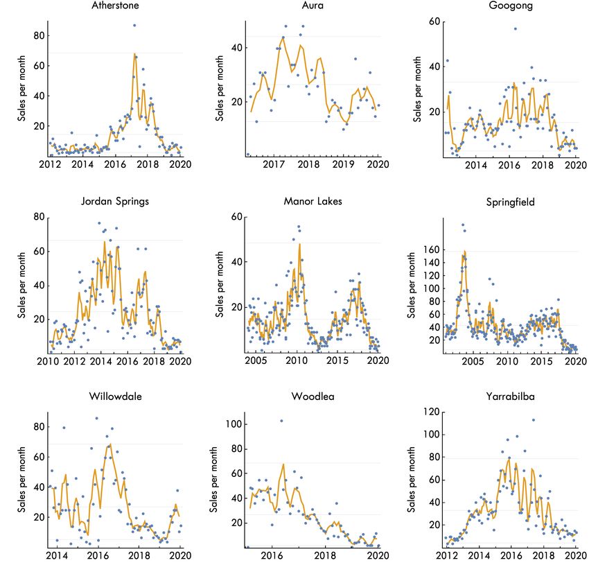
1      Introduction and motivation
Current academic and policy debates about housing prices often focus on planning and zoning
regulations (Ihlanfeldt, 2007; Quigley & Rosenthal, 2005; Rodrı́guez-Pose & Storper, 2020). The
mechanisms by which different planning regulations can affect the private choices of property
owners to develop housing are debated (Greenhalgh et al., 2021). Empirical approaches to
identifying links between planning and housing market outcomes necessarily rely on assumed
counterfactuals about the density, location, and importantly, the overall rate of new housing
supply in the absence of such regulations. Missing from the debate is an understanding that
even in the absence of planning regulations there is a constraint on the rate of new housing
supply known as the market absorption rate (Letwin, 2018; Murray, 2022).1 This rate is the
result of many property owners of candidate development sites in a region making choices about
when and how fast to develop new housing.
In this paper we take a closer look the private choices of property owners regarding the rate at
which they develop housing when there are no regulatory barriers on their choices—that is, after
major subdivision projects are approved and sales have commenced. Doing so highlights how
variation in the absorption rate is determined by market conditions, not planning policy settings.
This helps refine our understanding of the potential mechanisms by which planning systems may
affect private new housing supply choices.
The economic logic behind the market absorption rate is described in (Murray, 2022). Property
owners maximise their returns over time via their choice of development density and their choice
of development rate. Higher density does not automatically mean faster new housing supply
since the optimal rate of supply is not related to development density.2 When demand is rising,
increasing the rate at which undeveloped property assets are developed to new housing increases
overall returns. But when market demand is falling or thin, with few buyers at current prices,
slowing the rate of new housing development increases returns.3 A barrier to communicating
the market absorption rate concept is that the value to delaying development is difficult to see.
After all, it can seem odd that housing developers will voluntarily slow their rate of new housing
production even though they make money from selling new homes.
The main contribution of this article is to present new market absorption rate metrics that show
the variability of new housing supply and the economic payoff from varying housing production
in response to market conditions. The metrics are as follows.
    1. Development rate ratio (DRR) – average production rate to peak rate ratio
    2. Development rate variability (DRV) – minimum production rate to peak rate ratio
    3. Delay premium ratio (DPR) – average minus minimum price divided by minimum price
    4. Delay premium variability (DPV) – maximum minus minimum price divided by minimum
       price
    1 TheUnited States Census Bureau adopts this language in their Survey of Market Absorption of New Multi-
family Units (SOMA), which describes the rate that new multi-family units are rented or sold into the market.
   2 This can be seen by imagining a project with 100 approved dwellings selling at 5 per month. While selling,

the project is granted a new approval to double the density of later stages so that there are now 125 potential
dwellings in the project. If this future density change increases the current rate of sales, then the previous sales
rate was already sub-optimal.
   3 Other factors like interest rates (the return on the cash gained after a sale), taxes on land ownership (that

reduce the return to retaining ownership of undeveloped land), and the ability to vary the density of development
in the future (a flexible planning system can make delay more profitable by allowing higher density in the future,
increasing the return to delay), all can have small effects on this optimal rate.

                                                         2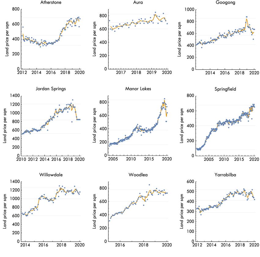
These metrics can be applied to major housing projects after approval to make visible how
the absorption rate regulates the pace of new housing and answer the question of why housing
developers choose to slow their rate of supply.
The DRR and DRV metrics describe the distribution of housing supply rates relative to their
peak rate. The peak rate demonstrates a rate of supply that is possible. Deviations below this
rate are private choices of property developers and the size of this deviation on average and at the
extreme is captured in these metrics. The DPR and DPV metrics describe the price distribution
over a project life relative to the minimum price in that project. Since the minimum price sold
reflects a profitable choice, deviations above this price reflect gains from delaying sales to future
periods with higher prices rather than selling all new housing at a set price as quickly as possible.
Both benchmarks for these metrics—the peak rate of supply and the minimum price—reflect
common arguments about how housing developers will sell as quickly and cheaply as possible but
for planning and zoning regulations. With a heated policy debate taking place in many countries
facing quickly-rising dwelling prices, simple metrics like these that can be easily understood by
a broad audience are valuable for communicating key the importance of the absorption rate
concept for housing supply policy.
For example, using these metrics we show that in a sample of large housing projects in Australia
with over 3,000 dwellings approved and sales data for at least five years, the average DRR is
about 34%, and the DRV is 7%. This is an enormous amount of variability in response to market
conditions, not planning regulation. We also show that varying the sales price over time increased
prices received in these projects by 82% on average (the DPR) compared to a counterfactual of
setting the price based on cost at the outset and selling all new dwellings at that minimum price.
Potential economic gains to delay can be large, with a 204% increase in price available if all new
dwellings were sold at the highest observed price rather than the lowest price over the project
life (the DPV).
To determine the robustness of this approach to understanding variation in the absorption rate
we also apply the metrics to housing development company data and to city planning data.
Doing so helps determine whether a similar level of variation to that seen at a project level also
occurs at higher levels of aggregation, like cities and companies, and hence housing markets as a
whole. These results are consistent with the project level data.

2     Relevant literature and policy context
Unlike previous housing booms, the 2000s housing boom led to a new focus on explanations from
the supply side of housing markets, which became broadly popular in the late 2010s as housing
markets recovered globally from the 2008-09 bust. Glaeser (2018) summarised the static cost-
based supply-side approach that has been widely adopted in these debates and informs many
recent academic debates.4
A parallel economic literature has taken a more dynamic approach to the question of housing
supply (Capozza & Li, 1994; Murphy, 2018; Murray, 2022; Guthrie, 2022). Unlike the static
cost-based analysis that focuses on optimal density, this research focuses more on the rate of
supply and the inter-temporal trade-off between developing more housing now or later.
Unfortunately, the concepts of density, location, and the rate of supply (the absorption rate)
   4 Such as in Urban Studies in 2021 (Rodrı́guez-Pose & Storper, 2022; Manville et al., 2022) and elsewhere (Been

et al., 2019).

                                                        3
are often conflated, hindering communication and understanding when different concepts are
applied. For example, upzoning an area can increase the density of development that occurs in
that area, but it may also shift development to that area away from neighbouring areas, with
potentially little or no impact on the total rate of housing supply across all areas.
This academic debate is closely tied to a policy debate about the effect of planning regulations
on new housing production. In the United Kingdom, the Barker Review of 2004, and Letwin
Review of 2018 both focussed on supply and planning regulation. In New Zealand, Auckland
City Council conducted a widespread major upzoning with their Unitary Plan in 2016, motivated
by supply-side arguments. In Australia, the 2022 Parliamentary Inquiry into Housing Supply
(the Falinski Inquiry) focussed on planning regulation and prices. These reviews occasionally
note the existence of the market absorption rate as a constraint on the rate of new supply, but
usually dismiss it. For example, during the Falinksi Inquiry, housing developers under oath said
that “rezonings won’t necessarily lead to lower housing prices” (Standing Committee on Tax and
Revenue, 2021). Before that, the Letwin Review concluded as follows.
...it would not be sensible to attempt to solve the problem of market absorption
rates by forcing the major house builders to reduce the prices at which they sell their
current, relatively homogenous products. This would, in my view, create very serious
problems not only for the major house builders but also, potentially, for prices and
financing in the housing market, and hence for the economy as a whole.
(Letwin, 2018, pp.8-9)
The absorption rate is a key issue in both the academic and policy debates, but one that is
ignored, overlooked, or assumed away. Finding a way to shine a light on this important concept
can help progress both debates and improve our understanding of housing markets.
3 Metrics and their interpretation
In this section, we note how each absorption rate metric answers a specific question. describe
how each metric can be applied to property sales data, and briefly note how the metric can be
interpreted in the context of housing supply policy debates.
3.1 Development rate ratio (DRR)
How fast did housing development occur compared to how fast it could have if all
housing was developed at the maximum observed rate?
The development rate ratio (DRR) is the ratio of the average production rate to the maximum
rate (see Equation 1). We use both the average monthly rate of sales over a three-month rolling
window and over a twelve-month window to smooth out any idiosyncratic variation. Sales can
be used as the measure of the speed of development in the case of build-to-order model (as is
the standard in Australia, for example) or new rentals in the case of build-to-rent models (as is
common in multi-family housing in the United States, for example). Both measures capture the
mechanism by which the rate of new housing supply is managed based on market conditions.
A lower number indicates that the new housing development proceeded more slowly than was
demonstrated to be possible in the observed sales or new rentals.
Average production rate
DRR = (1)
Maximum production rate
4This metric is a sense-check for claims that new housing is being built as fast as the planning
system allows. Once a subdivision or apartment building is approved by the planning system, only
the private choices of the developer determine how fast the approved new housing is developed.5
A DRR at, or close to, one means that the project was built near its maximum rate over its life.
However, a low DRR suggests that market choices lowered the rate of supply below what was
possible. For example, a DRR of 0.5 means that the rate of supply was on average half as fast
as it could have been. Or described differently, it is how much shorter the project timeframe
could have been if maximum production rates were sustained; a 10 year project with a DRR of
0.5 could have been completed in 5 years.
3.2 Development rate variability (DRV)
How much slower will developers produce housing compared to the maximum rate?
Development rate variability (DRV) is the ratio of the minimum production rate to the maximum
rate (as per Equation 2). Again, we use here the average monthly rate over three-month and
twelve-month rolling windows. The DRV shows the observed extent that private property owners
are willing to slow the rate of production in response to the market conditions even from approved
projects already under development. Like the DRR, rental rates or sales rates can be used
depending on the relevant market.
Minimum production rate
DRV = (2)
Maximum production rate
Calculating the DRV for a range of projects in a region provides evidence about the degree to
which the rate of new housing supply over time is being regulated by market conditions rather
than planning. For example, if the DRV for a range of projects was seen to be in the range of
0.05 to 0.20, then market conditions are generating variation in the rate of supply by a factor of
5 to 20 times.
3.3 Delay premium ratio (DPR)
How much higher are actual prices received compared to the minimum price?
The delay premium ratio (DPR) is the difference between the average price of dwellings in a
project and the minimum observed price as a ratio of that minimum price (see Equation 3). We
use three-month moving averages of price to remove noise.
Average price − Minimum price
DP R = (3)
Minimum price
The DPR metric highlights the economic gains available from regulating the rate of sales to
ensure they across time periods where prices are higher rather than selling as fast as possible at
the minimum price (usually the initial price). For example, a DPR of 0.5 means that the average
price, and hence revenue, was 50% higher than the minimum price over a project life. It would
also suggest that pricing of new dwellings is not based on costs and that controlling the rate of
5 Apartment projects often cannot be built in stages, but they will be sold over a long time period, usually
many years, with sales occurring before constructions (to hit pre-sale risk hurdles), during construction, and often
for years post construction. Even though construction itself might take 1-2 years, the sales make take 3-5 years,
or longer.
5supply to sell at opportune times vastly increases project revenues. It highlights the potential
magnitude of the economic incentive to produce new housing slower than is possible under given
planning conditions.
To further understand the magnitude of this incentive, it must be noted that profit margins are
usually a small share of the price, normally in the 10% to 30% range. In terms of the variation
in net economic returns, selling at an average price 50% higher than the minimum over a project
life, assuming a profit margin of 20% if sold at the minimum price, is a more than tripling of
profits (3.5 times the profit). How big these gains are in the dollar value terms can be calculated
by multiplying the DPR by the minimum price and by the number of dwellings in a project.
3.4 Delay premium variability (DPV)
How much higher is the maximum price received compared to the minimum price?
The DPV metric shows the full range of variation in price over a project lifetime as a ratio of
that minimum price (see Equation 4). We again use three-month moving averages of price to
remove noise.
Maximum price − Minimum price
DP V = (4)
Minimum price
Like the DPR, the DPV highlights the scale of economic gains from delay, though in this case it
shows the size of the full range of price changes over a project life. A DPV of 0.9, for example,
means that the maximum price received was 90% higher than the minimum price. If all new
dwellings were sold at the maximum price instead of the minimum this is also the proportional
gain in revenue available. In situations where the price at the end of the project is highest, and
lowest at the beginning, it shows the size of the value gains had the whole project to date been
delayed to instead start in the latest high value period, and hence points to the value of delaying
housing projects altogether.
4 Application of metrics
For this demonstration we use complete Australian property sales records sourced from data re-
seller CoreLogic. Our available data covers the period January 2001 to January 2020 in the major
states of Queensland, New South Wales and Victoria. The ultimate sources of these records are
state land titles offices, where property transaction dates and prices are recorded.
We focus on major land subdivisions with over 3,000 housing lots that were actively selling for
more than five years during the period of data coverage. Focussing on land alone neatly shows
the net financial incentives without having to account for construction costs of new homes to
determine the net gains from property development. We chose nine major housing subdivisions
spread across the major states on the outskirts of the capital cities. Descriptions of each subdi-
vision project are Table 1. These projects were chosen because of their size (being a substantial
share of local new housing supply), their location (on the fringes of capital cities) and because
they are predominantly land subdivisions, and hence prices can be applied on a per land area ba-
sis to the DPR and DPV counterfactuals for the subset of sales that are land only (i.e. prices for
these two metrics are on a dollar-per-square-metre basis and total production for these metrics
is measured by land area not lots).
6Table 1: Description of major subdivision sample projects
Project State Start Total Lots in Owner Type Location
name year lots sample
Atherstone VIC 2012 4,300 1,372 Lendlease Public 40km W of Melb.
Aura QLD 2016 >20,000 1,188 Stockland Public W of Caloundra
Googong NSW 2012 5,961 1,454 Mirvac Public Outskirts of ACT
Jordan Springs NSW 2010 4,800 2,890 Lendlease Public 55km W of Syd.
Manor Lakes VIC 2004 4,996 2,832 D.F.2 Private 37km W of Melb.
Springfield QLD 19941 >32,000 9,814 S.L.C.3 Private 32km SW of Bris.
Willowdale NSW 2013 3,722 2,098 Stockland Public 40km SW of Syd.
Woodlea VIC 2015 6,584 1,563 V.I.P. 4 Private 39km W of Melb.
Yarrabilba QLD 2011 >17,000 3,165 Lendlease Public 38km S of Bris.
1
Data from 2001 only. Subdivision began in 1994 and is ongoing as of 2022.
2
Denniss Family.
3
Springfield Land Corporation often in conjunction with other developers for delivery of project stages.
4
Victoria Investments and Properties Pty Ltd (partnered with Mirvac).
To select the relevant new property sales data from the complete record of property sales, latitude
and longitude property coordinates are used to ensure sales reflect new lots falling with the
subdivision boundary. Sales dates are chosen to be after the start date of the first stages of each
project, with only the first sale of each lot being used. Lot sizes are selected to include only those
falling within the range of sizes in the subdivision plan. In many cases the projects included
townhouses and apartments and these sales were not included. All projects remained in progress
as of the end of 2020. We use the data to calculate the absorption rate metrics to sales contracted
prior to January 2020, as investor publications of some of the publicly-listed companies in our
sample show that during financial year 2020-21it became common for new sales contracts to be
signed, and deposits taken, that are conditional upon completion of future stages that were not
ready for settlement.
We also note that there is likely some missing data in our sales records. If we compare this sales
data and the reported sales in financial reports of the publicly-listed companies that own some
of the sample projects, the sales data is generally lower than the company-reported reported
sales and settlement data. For example, Mirvac, owner of Googong and Woodlea projects, has
reported project level sales and/or settlements in some of their end of year results. In 2016 the
company reported 889 sales in Woodlea and only 415 settlements, while Corelogic records have
560 sales that year. In Googong that year the company reported 343 sales and 525 settlements,
while the Corelogic records showed 208 sales. There is clearly both a long delay between sales
and settlement, and smoothing of sales into settlements across different time periods. This
makes sense, as listed companies have incentives to stabilise revenue streams by smoothing out
settlements, when full payments occur, and to stabilise rates of physical construction activity.
To determine whether potential missing data is undermining the accuracy of the metrics we also
look at company data in Section 5 and city level data. With additional diversity of supply at
these higher levels of aggregation, they represent upper bounds of project level metrics, and a
close correspondence would imply that market as a whole has similar absorption rate constraints
as individual projects.
7Table 2: Application of metrics to selected major subdivisions
Project DRR DRR DRV DRV DPR DPV DPR DPV DPR
3 m. 12 m. 3 m. 12 m. 3 m. 3 m. × prod. × prod. per lot
($m) ($m) ($’000)
Atherstone 0.21 0.46 0.04 0.14 0.42 1.15 61 170 44
Aura 0.45 0.57 0.29 0.39 0.15 0.37 36 89 30
Googong 0.42 0.47 0.08 0.11 0.53 1.06 193 385 133
Jordan Springs 0.34 0.40 0.04 0.07 0.59 1.33 333 753 115
Manor Lakes 0.29 0.37 0.03 0.07 1.25 4.13 215 711 76
Springfield 0.25 0.44 0.04 0.12 3.03 7.27 1,201 2,880 122
Willowdale 0.38 0.46 0.08 0.23 0.53 1.05 228 455 108
Woodlea 0.32 0.39 0.03 0.07 0.46 1.23 98 264 63
Yarrabilba 0.37 0.42 0.06 0.07 0.43 0.78 161 290 51
Mean 0.34 0.44 0.07 0.14 0.82 2.04 83
!
Adjacent to the ACT border and hence a satellite of Canberra.
∗
Data from 2001 only. Subdivision began in 1994 and is ongoing as of 2022.
In Table 2 we summarise the four absorption rate metrics. The 0.34 mean DRR shows that the
average rate of new housing production is a third of the demonstrated maximum possible rate,
which is a little higher when using twelve month moving average rate of monthly sales, at 0.44.
A DRR value this low suggests that the rate of new housing production is not being maximised
but managed. This is further shown by the low DRV metric across all projects. Looking at three
month windows, the DRV was 0.07 on average, though this would be only 0.05 if the newest
project, Aura, was excluded from the sample. Even using a twelve month average rate, the DRV
was 0.14 on average, and 0.11 if Aura is excluded. This means that some years the rate of sales
is seven to nine times higher than other years during a project life.
To show visually the patterns the DRR and DRV metrics are capturing, Figure 1 shows a
histogram of the monthly rate of sales for all projects combined. The strong left skew is not
expected in a scenario where planning the binding constraint on the rate of new supply. If that
were true, there would be a strong right skew towards supplying new homes near the maximum
rate from approved projects.
Moving to the metrics of the premium from delay, we see a delay premium ratio (DPR) of 0.82
across these sample projects. This implies that the price received per square metre on average
across all new land sales was 83% higher than the minimum sale price. If we assumed that the
minimum price covered costs, this metric highlights just how large the gains are for landowners
from managing their production rates over time to both avoid flooding the market to decrease
prices, and selling in later periods when prices are higher. In terms of the dollar value of this
additional revenue, these were typically in the tens to hundreds of millions (third to last column).
It is easy to see how such large values arise. For example, an extra $200/sqm for a 400sqm lot is
$80,000. Multiply this by just one hundred lots and that is already $8 million. Prices per square
metre of land were on average $653/sqm in this sample of projects, and varied by $517 between
their lowest and highest prices. If profit margins are 25% at the minimum price, then a DPR of
0.83 implies a 332% increase in profits by managing sales rates to achieve higher prices later .
8Figure 1: Distribution of monthly sales rates in sample projects combined
Indeed, the DPV of 2.04 shows that the difference in revenue between selling all lots that max-
imum price rather than the minimum would have generated 204% more revenue. If all new
housing lots are sold quickly at the initial price, these higher priced future sales opportunities
are missed. This also shows the payoff in terms of the change in the value of land for a neighbour-
ing property owner who has the option to develop but chooses instead to wait. The same applies
to staging of these project themselves. Future stages of this sample of projects, if considered
as their own individual projects, will earn a price 204% higher than the first stages. Longer
term projects, such as Manor Lakes and Springfield, saw much higher DPR and DPV metrics,
as expected given the housing price growth seen in Australia since 2000.s
The additional revenue obtained in these projects because of selling above the minimum price is
exceptionally large in dollar terms, ranging from $60 million to $1.2 billion. On a per lot basis
across all projects the average lot was sold $83,000 above the corresponding minimum price in
that project.
We can look in more detail at one of the projects, Atherstone, to see the underlying patterns
reflected in these metrics. In Figure 2 we see in the top left panel the land price per square
metre over time during the life of the project. When the project began the price was around
$400/sqm in 2012. It stayed relatively flat until 2017 when it jumped to around $600/sqm. This
was a period in which sales increased from five per month to over 60 per month, a twelvefold
increase (top right panel). The relationship between price growth and supply is more clear in
the bottom left panel, and the low average rate of supply alongside huge variation in it is shown
in the bottom right histogram.6 Plots of the rate of new lot sales and land prices in each project
are in Figures A1 and A2 of the Appendix.
6 Land price growth and sales rates in the bottom left panel are plotted after applying a gaussian filter over a
three month window to each variable.
9Figure 2: Sale rate and prices for the Atherstone project (Victoria)
5 Alternative metric applications
Though we focus on approved housing projects to highlight how variation in the rate of supply
arises after planning approvals, the absorption rate metrics can also be applied to other data.
Doing so reveals whether larger markets operate similarly to individual projects in terms of the
absorption rate being heavily regulated by market factors.
5.1 Development company data
Using company data directly as the basis for absorption rate analysis can be done using state-
level residential sales data reported by Stockland, a publicly-traded company that has projects
in our main data sample. They are the only company that reports quarterly sales data across
the four states they operate in, which they have done since 2012 for all types of dwellings within
their residential projects. The DRR and DRV absorption rate metrics applied to this data are
10in Table 3, using both quarterly and annual periods, and the quarterly rate of new housing lot
production in each state is in Figure A3 of the Appendix. These metrics reveal less variability
than the DRV and DRR using 3 month average rates at a project level from Table 2, which is
expected as there is a diversity of projects in each state.
What this exercise shows is that even across many projects in a state, the variability in the rate
of supply is quite large, with the minimum rate of sales usually being only 22% of the maximum
rate, and the average rate about half, suggesting a large degree of sensitivity to market conditions.
Even taking a whole year period, the average year has 60% of the sales of the peak year, and
the minimum year has 34% in each state. Given that this applies to across 10 projects in each
state on average suggests that the variation in the rate of supply at a project level must me
much larger, implying much lower DRR and DRV metrics. As such, these measurements allay
concerns about any missing data in the property sales records being a major factor creating an
abnormally low value of the DRR and DRV metrics.
The interpretation of the metrics applied at this scale is less clear, however. Planning may
influence the variation in sales. But it is nevertheless interesting to read the company source
reports, as they make no mention of planning rules being the cause of the rate of sales. These
reports instead note that market conditions are the most important determinant of the rate of
sales.
Table 3: Company level housing production
State Projects DRR DRR DRV DRV
in state Quarterly Annual Quarterly Annual
Queensland 18 0.68 0.74 0.41 0.55
New South Wales! 7 0.39 0.46 0.11 0.20
Victoria 10 0.52 0.65 0.18 0.32
Western Australia 6 0.46 0.56 0.19 0.29
All states total 41 0.66 0.75 0.37 0.53
Mean of states 10 0.51 0.60 0.22 0.34
!
Includes Australian Capital Territory
Data from 1Q2012 to 4Q2021 from annual reports
5.2 Aggregate city data
Another application for these absorption rate metrics is city-wide planning data. This can show
the degree to which variation in new dwelling supply arises from market choices to develop
housing out of the stock of approved projects. Small DRR and DRV metrics would imply a high
degree of variation that is hard to explain based on planning rules rather than market conditions
regulating the rate of new housing supply. They would instead support the idea that regional
markets as a whole face similar absorption rate constraints to individual projects.
In Table 4 we show the DRR and DRV using the quarterly new housing lot registration data
for councils in south east Queensland from March 2002 to December 2021 for both attached and
detached dwellings.
Notice that even at a regional market level (council area rather than subdivision project area)
that there is a similar degree of variation to that seen in individual major subdivision projects.
11The DRR is just 0.39 across all council areas, and the mean DRV of 0.10 implies that the
maximum rate of new housing production in a quarter is ten times the minimum. Plots of the
quarterly rate of new housing lot registrations (attached and detached) in each council area are
in Figure A4 of the Appendix.
To show that the stock of approvals was not a factor at play, we show in the final column of Table
4 the mean ratio of quarterly lot completions to the stock of approvals. The data on the stock
of approvals, however, is only available for detached housing lots, so we only include detached
lot and approvals data. The amount of dwellings in the approved pool in was typically 10 to
20 times larger than the quarterly lot completions, and grew over this period for nearly every
council, suggesting that the approval process was not a constraint on these rates of supply. At
a city level, the pace of new housing appears to market conditions with a similar amount of
variation as individual housing project.
Table 4: Council lot registration absorption metrics
State DRR DRV Mean ratio
Quarterly Quarterly (qtrly new lots per
approved stock)
Brisbane 0.43 0.20 0.11
Gold Coast 0.48 0.12 0.09
Ipswich 0.41 0.07 0.07
Lockyer Valley 0.31 0.01 0.05
Logan 0.48 0.13 0.08
Moreton Bay 0.64 0.30 0.10
Noosa 0.22 0.01 0.11
Redland 0.41 0.06 0.10
Scenic Rim 0.26 0.02 0.05
Somerset 0.17 0.00 0.04
Sunshine Coast 0.48 0.12 0.09
All councils total 0.61 0.30 0.07
Mean of councils 0.39 0.10 0.08
Data from 1Q2001 to 4Q2021 from Queensland Government Statisti-
cian’s Office
Lot registrations for DRR and DRV are for detached and attached lots.
Mean ratio of new lots to stock of approved lots is for detached only, as
stock of approved lots is not available for attached dwellings.
6 How these metrics contribute to current debates
Taken together, this suite of new metrics highlights the central role of the market absorption rate
in determining how fast new housing is produced. Their application to major housing projects
in Australia shows that housing producers are extremely sensitive to market conditions in their
choice of the rate of new supply, and that the financial gains to adapting sales rates and prices
to market conditions are substantial. We show that our approach to using property sales records
12matches closely the approach of using company sale records, where available, though there is
some discrepancy about the overall extent of variation in the rate of sales (the DRV). Adding
to this, we have applied the new absorption rate metrics at a company level to show the high
degree of variation in the rate of new supply even at this aggregate level. A further level of
aggregation to council areas shows similar variability in the rate of supply to that seen at a
project level. These new metrics can be applied in many ways to illustrate that the absorption
rate of new housing appears predominantly market determined rather than the result of planning
regulations.
The fact that the rate of supply on major approved projects is typically far below the maximum,
and varies by a factor of 14 or more, suggesting that any mechanism by which planning regulations
lead to housing price effects must deal with an additional constraint in the form of the absorption
rate.
If there is an optimal absorption rate, individually and collectively for new housing in a market,
how might planning regulations affect this rate? This is a missing question in both the academic
and policy debate. But with this new way of communicating the importance of the absorption
rate and the economic motive behind it, perhaps such debates can quickly evolve.
To progress these potentially more fruitful debates we briefly outline a handful of potential
arguments about the relationship between planning regulations and the market absorption rate,
and address each by drawing on the evidence generated by these new metrics.
One potential line of reasoning is that the planning system is not responsive enough, and hence
delays for planning approvals cause delays to supply when market conditions turn favourable,
and when market conditions revert there is not incentive to “catch up” with supply. However, the
argument implies that market housing producers are incapable of investing in a buffer stock of
approved sites to accommodate variability in demand. Indeed, the DRR and DRV show that the
market does invest in large buffer stocks of approvals, as does the evidence of council approvals
in Table 4. Even if this were an accurate representation of how planning affected the absorption
rate, then the quantity effects would be extremely small even over decades, as there are few
infrequent boom periods.
Another argument is that planning or zoning reduces supply because only a small share of
developable sites are economically viable, creating market power. Large scale rezoning creates
many more viable sites (where price exceeds development cost) resulting in faster production
because of price competition. This is the mechanism Glaeser (2018) describes as the way planning
regulations modify the “supply curve”. However, the housing development market is competitive
by any standard measure, such as the Herfindahl-Hirschman Index (HHI). In 2018 the top twelve
Australian housing developers supplied only about 9% of new homes nationally, suggesting a
HHI in the range of 0.0016 to 0.0025 (Murray, 2020).7 This is below the tenth percentile of
HHI estimates for Australian industries, indicating an extremely competitive market (Bakhtiari,
2019). Furthermore, the same high property prices, unequal access to property ownership, and
enormous land price cycles happened historically before the invention of zoning, and were defining
characteristics of the property markets of the 1800s in countries like Australia the United States
and United Kingdom. Market power seems inherent to property systems (Posner & Weyl, 2017).
Lastly, an argument might be that without planning regulations (or zoning) the same variability
in the absorption rate will occur but at a higher average rate. However, if at every point in time
7 The upper end of the range is based on the next dozen housing developers being equally as large as the first
dozen, before market share drops below 1%, and the lower end is if market share of the remaining firms are all
below 1%.
13the market wishes to develop housing faster, it could, as the variation in the absorption rate
shows what is possible. This line of reasoning relies on the idea that under the same market
conditions and the freedom to choose the rate of supply, the very existence of a zoning system
changes the optimal rate. It appears to be a competition argument in disguise.
7 Conclusion
New ways to communicate the market absorption rate and the economic motives behind it are
an important step in progressing academic and policy debates about planning, housing supply
and prices. By highlighting the variability of the absorption rate with new metrics that can be
applied at a project level, company level, or city level, a clearer picture of how market conditions
regulate the supply of new housing emerges. Future studies of planning regulations and their
effects on housing supply must address the mechanism by which planning regulations affect the
absorption rate.
14References
Bakhtiari, Sasan. 2019 (September). Trends in Market Concentration of Australian Indus-
tries. Research Paper 8/2019. Department of Industry, Innovation and Science. Australian
Government.
Been, Vicki, Ellen, Ingrid Gould, & O’Regan, Katherine. 2019. Supply skepticism:
Housing supply and affordability. Housing Policy Debate, 29(1), 25–40.
Capozza, Dennis, & Li, Yuming. 1994. The Intensity and Timing of Investment: The Case
of Land. The American Economic Review, 84(4), 889–904.
Glaeser, Edward, & Gyourko, Joseph. 2018. The Economic Implications of Housing
Supply. Journal of Economic Perspectives, 32(1), 3–30.
Greenhalgh, Paul, McGuinness, David, Robson, Simon, & Bowers, Kathryn. 2021.
Does the Diversity of New Build Housing Type and Tenure Have a Positive Influence on
Residential Absorption Rates? An Investigation of Housing Completion Rates in Leeds City
Region. Planning Practice & Research, 36(4), 389–407.
Guthrie, Graeme. 2022. Land Hoarding and Urban Development. The Journal of Real Estate
Finance and Economics.
Ihlanfeldt, Keith R. 2007. The effect of land use regulation on housing and land prices.
Journal of Urban Economics, 61(3), 420–435.
Letwin, Oliver. 2018 (October). Independent Review of Build Out Rates - Final Report. Tech.
rept. Ministry of Housing, Communities and Local Government.
Manville, Michael, Lens, Michael, & Monkkonen, Paavo. 2022. Zoning and affordabil-
ity: A reply to Rodrı́guez-Pose and Storper. Urban Studies, 59(1), 36–58.
Murphy, Alvin. 2018. A dynamic model of housing supply. American Economic Journal:
Economic Policy, 10(4), 243–67.
Murray, Cameron K. 2020. Time is money: How landbanking constrains housing supply.
Journal of Housing Economics, 101708.
Murray, Cameron K. 2022. A Housing Supply Absorption Rate Equation. The Journal of
Real Estate Finance and Economics, 64(2), 228–246.
Posner, Eric A, & Weyl, E Glen. 2017. Property is only another name for monopoly.
Journal of Legal Analysis, 9(1), 51–123.
Quigley, John M, & Rosenthal, Larry A. 2005. The effects of land use regulation on the
price of housing: What do we know? What can we learn? Cityscape, 69–137.
Rodrı́guez-Pose, Andrés, & Storper, Michael. 2020. Housing, urban growth and inequal-
ities: The limits to deregulation and upzoning in reducing economic and spatial inequality.
Urban Studies, 57(2), 223–248.
Rodrı́guez-Pose, Andrés, & Storper, Michael. 2022. Dodging the burden of proof: A
reply to Manville, Lens and Mönkkönen. Urban Studies, 59(1), 59–74.
Standing Committee on Tax and Revenue. 2021. Housing affordability and supply in
Australia (26/11/2021 transcript). Tech. rept. Parliament of Australia.
15Appendix
Figure A1: Sales rates in subdivision sample projects (three month moving average line)
16Figure A2: Prices of new detached housing lots in subdivision sample projects ($/sqm)
17Figure A3: New housing lot production rate, attached and detached, Stockland state level
18Figure A4: Quarterly new housing production (attached and detached) in Queensland councils
19You can also read