WP/21/85 Does a Wealth Tax Improve Equality of Opportunity? Evidence from Norway - by Kristoffer Berg and Shafik Hebous
←
→
Page content transcription
If your browser does not render page correctly, please read the page content below
WP/21/85

Does a Wealth Tax Improve Equality of Opportunity?
                           Evidence from Norway

                      by Kristoffer Berg and Shafik Hebous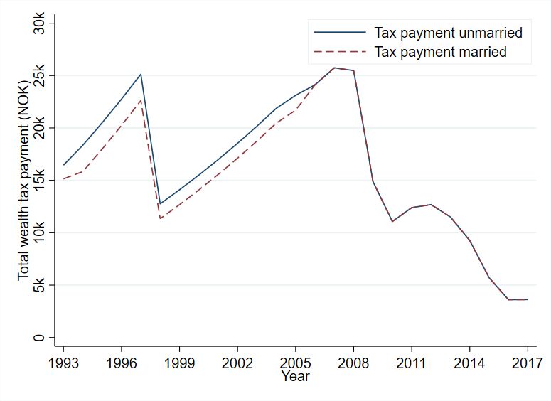
2

© 2021 International Monetary Fund                                                                    WP/21/85

                                           IMF Working Paper

                                         Fiscal Affairs Department

          Does a Wealth Tax Improve Equality of Opportunity? Evidence from Norway

                          Prepared by Kristoffer Berg and Shafik Hebous 1

                            Authorized for distribution by Alexander Klemm

                                                March 2021

    IMF Working Papers describe research in progress by the author(s) and are published to elicit
    comments and to encourage debate. The views expressed in IMF Working Papers are those of the
    author(s) and do not necessarily represent the views of the IMF, its Executive Board, o r IMF
    management.

                                                  Abstract

Does parental wealth inequality impact next generation labor income inequality? And does a
tax on parental wealth affect the labor income distribution of the next generation? We tackle
both questions empirically using detailed intergenerational data from Norway, focusing on
effects on wages rather than capital income. Results suggest that a net wealth of NOK 1
million increases wages of the children by NOK 14,000. Children of wealthy parents also have
a higher labor income mobility. The estimated hypothetical wage distribution without the
wealth tax is more unequal. Moreover, suggestive evidence indicates parental wealth is
associated with higher labor risk taking.

JEL Classification Numbers: D31, D63, H24

Keywords: Wealth Tax, Equality of Opportunity, Parental Wealth, Income Mobility, Inequality,
Redistribution

Authors’ E-Mail Addresses: kristoffer.berg@econ.uio.no; shebous@imf.org;

1
 We received helpful comments from Giacomo Brusco, Jean-Marc Fournier, Edwin Leuven, Michael Keen, Paolo
G. Piacquadio, Kjetil Storesletten, Magnus E. Stubhaug, Kasper Kragh-Sørensen, Marius Ring, Thor O. Thoresen,
and Jean-Francois Wen, and seminar and conferences participants at the IMF and the University of Oslo.
3
Content Page
Abstract ____________________________________________________________________________________________________2
I. Introduction _____________________________________________________________________________________________4
II. Norwegian Wealth Tax and Data ___________________________________________________________________7
A. Norwegian Wealth Tax _________________________________________________________________________________ 7
B. Data ______________________________________________________________________________________________________ 8
III. Empirical Approach __________________________________________________________________________________9
A. IV Estimation and Clarifying the Potential Bias _______________________________________________________ 9
B. Specifications __________________________________________________________________________________________ 11
IV. Resutls________________________________________________________________________________________________ 13
A. Main Restuls _____________________________________________________________________________________________ 3
B. Extensions______________________________________________________________________________________________ 15
V. Conclusion____________________________________________________________________________________________ 18
References _______________________________________________________________________________________________ 19
Appendix_________________________________________________________________________________________________ 21
Figures
1. Wealth Tax Rates and Payments _______________________________________________________________________ 7
2. Parental elath, Wgae, and Capital Income ____________________________________________________________ 9
3. Counterfactual Income Distribution in the Absence of a Wealth Tax _____________________________ 15
4. Labor Income Dispersion and Parental Wealth Levels _____________________________________________ 17
Tables
1. Main Resutls ___________________________________________________________________________________________ 14
2. Heterogeneous Effects across Wealth Levels _______________________________________________________ 16I Introduction
At the heart of the current debate about sharp and increasing wealth inequality is its potential
impact on income inequality in the next generation—an aspect reflecting equality of opportunity.1
If children of wealthy parents are not only more likely to earn higher capital income—as suggested
in the literature2 —but also higher labor income than peers from less wealthy families with otherwise
similar characteristics, then parental wealth entails a privilege that reduces equal prospects of
earning income. In this sense, a causal effect of parental wealth on intergenerational wages and
labor income mobility reflects better opportunities created by the stock of parental wealth.
The debate on wealth inequality has triggered a strong interest in—and a growing recent litera-
ture on—wealth taxation. Thus far, however, the literature has not provided evidence regarding the
question: does a tax on parental wealth affect the labor income distribution of the next generation?
Arguably, it is a challenging question to answer, not least in face of demanding data requirement to
establish links between parental wealth, children income when grown up, and a real-world wealth
tax.
This paper empirically studies the effects of parental wealth, and its taxation during childhood,
on adult income in Norway. The wealth tax in Norway—currently one of the few wealth taxes in
the world—has a relatively broad coverage, providing the advantage of studying a wide spectrum
of taxpayers beyond the superrich.3 Our research design focuses on cohorts born during 1978-1980
and estimates the effect of taxing the wealth of their parents in the late 1990s (i.e., when they were at
advanced stages in school) on their income in 2013-2017 (i.e., during adulthood). We focus on three
outcomes for these cohorts: i) the level of wage; ii) the position on the labor income distribution;
and iii) position on the labor income distribution relative to that of their parents—a measure of
intergenerational income mobility.
The identification of the causal effect of parental wealth on the income of the children relies
on two sources of variation: i) changes to the wealth tax rate in the late 1990s and early 2000s;
and, importantly, ii) different levels of taxation of the same level of wealth, depending on the
marital status. Specifically, we exploit that the wealth tax threshold and deduction of a married
couple filing jointly were higher than that for single filers with the same level of wealth. Thus, we
estimate an IV model using tax changes (due to marital status differences and tax law changes)
as an instrument for changes in net parental wealth.4 To address potential concerns about the
1 See,e.g., Piketty and Zucman (2014), Smith et al. (2020), and Boserup et al. (2018).
2 Fagereng et al. (2021)
3 See Scheuer and Slemrod (2020).
4 A similar strategy was used in Jakobsen et al. (2020) who focus on the elasticity of capital with respect to the
abolished Danish wealth tax.
4exclusion restriction (including the possibility that divorce can directly affect future income of the
children), we separately estimate the direct divorce effect on the income of the children from a
sample of taxpayers that are out of the scope of the wealth tax throughout the entire sample period,
and adjust our IV estimation accordingly. As we will explain later, this strategy plausibly provides
an upper bound of the divorce effect.
Our analysis yields two main results, consistent across the three considered outcome variables
and different rich sets of covariates to control for potential omitted variables bias. First, those
who grow up in families with higher levels of net wealth tend to have higher labor incomes,
controlling for the education and incomes of their parents as well as individual characteristics
including education. The benchmark estimates suggest that a net wealth of 1 million USD in
Norway increases future annual wages of the children by 14,000 USD, ceteris paribus. Second,
based on these point estimates, we estimate the counterfactual income distribution in 2017, in our
sample, in the absence of the wealth tax to answer the question: What would have happened to
the labor income distribution today had Norway not implemented a wealth tax in the late 1990s
and early 2000s? Our results suggest that the wealth tax has made the labor income distribution
less unequal—lowering the Gini coefficient by about 1 point. Moreover, results suggest that the
intergenerational labor income mobility is influenced by the stock of parental wealth, with children
from more wealthy families experiencing higher labor income mobility than those from less wealthy
families.
Extending the analysis to account for heterogeneous effects across wealth levels suggests that
the impact of the wealth tax on the labor income of the children is higher at middle levels of
wealth. Intuitively for the superrich, capital income plays a key role diminishing the importance of
employment income whereas low levels of parental wealth do not appear to significantly increase
the chances of improving the children position on the labor income distribution.
The questions as to how much and how (if at all) the income distribution should be made
more equal require normative analysis as, ultimately, optimal redistribution polices are dependent
on society’s preferences and the social welfare function. The positive analysis in our study, how-
ever, does inform policymakers by providing empirical evidence that a wealth tax is one policy
instrument that can lower the next generation income inequality.
Our paper leaves it for future research to closely study mechanisms through which the parental
stock of wealth impacts the labor income of their children. However, we do provide empirical
evidence pointing to directions for further research. Our results mute a potential education channel
as we control for higher education and the field of the study of the children.5 This prompts us to
5 Note also that affordability and access to high quality education is facilitated by the public education system in
5think of further mechanisms beyond human capital formation. We provide first empirical evidence
suggesting that one of those mechanisms is the risk profiles of decisions related to labor income.
For example, wealth can act as a private safety net. Results indicate heterogeneous returns to labor,
as higher levels of parental wealth are associated with a higher dispersion of labor income after
controlling for individual and parents’ characteristics. This finding complements recent evidence
on heterogeneous returns to capital as one explanation of intergenerational correlation in wealth
levels (Fagereng et al. (2021) and Benhabib and Bisin (2018)). In this context, our results explicitly
point to the role of the heterogeneity of labor income (in addition to capital income), associated
with different levels of parental wealth, in driving heterogeneous total wealth returns.
Our study links three strands of literature. The first is the empirical literature on wealth taxation,
which—as surveyed in Scheuer and Slemrod (2021)—mainly looks at two broad aspects: i) the
real effects of a wealth tax on capital accumulation (e.g., Jakobsen et al. (2020)); and ii) behavioral
(mostly evasion) responses as well as the revenue potential of various wealth tax designs (e.g., Saez
and Zucman (2019); Seim (2017); Bjørneby et al. (2020)). Secondly, a strand of the literature looks at
intergenerational or regional income mobility but with a focus on describing patterns in the data
without linking them to a wealth tax (e.g., Chetty, Hendren, Kline, Saez, and Turner (2014); Corak
(2013); Lee and Solon (2009); and Thoresen (2009)). Finally, a related growing literature studies
specific mechanisms of inequality of opportunity. For example, a series of papers—including
Chetty et al. (2020), Chetty, Hendren, Kline, and Saez (2014), and Chetty et al. (2018)—relate the
distribution of students’ earnings in their thirties to their parents’ incomes. They document, inter
alia, that low- and middle-income students attend selective schools at much lower rates than their
peers from higher-income families with the same test scores, but those that attend these schools
have similar long-term outcomes. This suggests that college attendance patterns have an upward
effect on income mobility.
This paper proceeds as follows. Section II summarizes the Norwegian wealth tax during the
sample period. Section III presents the identification approach. Section IV discusses the results.
Section V concludes.
Norway.
6II Norwegian Wealth Tax and Data
A Norwegian Wealth Tax
Today, Norway is one of a few OECD countries that levies a tax on the net wealth of individuals.6
The marginal wealth tax rate has varied considerably over time from a three-step progressive rate in
the mid-90s—reaching a rate of 1.5 percent—to a flat rate from the early 2000s—currently set at 0.85
percent (left panel of Figure 1). One specific feature in the Norwegian wealth tax is its relatively low
threshold, implying a significant number of taxpayers. The tax threshold currently is a net wealth
above NOK 1.5 million (about USD 174,000)—which is doubled for married couples—compared to
NOK 125,000 and NOK 150,000 for singles and married couples, respectively, in the early 1990s. In
1993, about 18 percent of Norwegian taxpayers were subject to the wealth tax, while in 2017 the
number had dropped to 10 percent.7
Figure 1: Wealth Tax Rates and Payments
(a) Top Marginal Wealth Tax Rate (b) Tax Payments: Married vs Unmarried
To illustrate differences in taxing the wealth based on marital status in the 1990s and early 2000s,
the right panel of Figure 1 shows tax payments over time for married and unmarried couples that
have the same the level of equally distributed wealth. For illustration, couples start with NOK
500,000 in 1993 (roughly USD 40,000 using 1993 exchange rate) and we increase the wealth at a
predetermined rate of 5 percent annually. Figure 1 displays larger differences in tax payments
between married and unmarried parents before 2006, which we exploit in our identification strategy
6 The Norwegian wealth tax was introduced in 1892. Currently, in OECD countries, in addition to Norway, e.g.,
Switzerland and Spain have a wealth tax. Ongoing discussions about a wealth tax are taking place in several countries
including the United States, Argentina, and South Africa.
7 See Bjørneby et al. (2020) and Ring (2020) for detailed descriptions of the Norwegian wealth tax.
7(see also Table A.1).
B Data
The source of the data is Statistics Norway’s databases including the Income Statistics for Families
and Persons which contains the Register of Tax Returns and other detailed information on indi-
viduals, enabling us to link parents with their children and trace their different sources of income
and their net wealth since 1993. Moreover, the database contains information about education
levels, including the field of study, the place of birth, and other characteristics. The Appendix
describes the definitions of all variables and presents detailed descriptive statistics in the sample
distinguishing between married and unmarried taxpayers (Tables A.2, A.3, and A.4). In 1993, the
average net financial wealth was 85 percent of the average wage. By 2017, the average net financial
wealth had risen to 135 percent of the average wage. Unsurprisingly, wealth is concentrated at the
top 10 percent wealthiest owned about half of all (positive) net wealth in Norway in 2017.
Figure 2 visualizes the main finding of the paper. It presents graphical evidence showing the
correlation between parental wealth in 1993-1999 and the percentiles of the income distribution of
the children in 2013-2017. The correlation patterns are estimated separately for wages and capital
income, controlling for characteristics including: parental wages in 1993-1999, birth in an urban
area, age of the wage earner, age and education of the parents. Figure 2 shows that high parental
wealth—during childhood—is associated with a better position in the labor income distribution
when grown up. Furthermore, confirming existing studies in the literature, the upward slopping
relationship is also observed between parental wealth and capital income.
8Figure 2: Parental Wealth, Wage, and Capital Income
Note: The binned scatterplot shows the estimated relationship between net parental wealth in 1993 and the
position on the labor income or capital income distribution in 2010-2017, controlling for parents and individual’s
characteristics including education.
III Empirical Approach
A IV Estimation and Clarifying the Potential Bias
The main identification strategy is to compare wage outcomes of children of married, unmarried,
and divorced parents over time. These groups were taxed differently on their wealth throughout
the 1990s and early 2000s. Furthermore, we explicitly account for a potential direct effect of divorce
on the income of the children.
Let Yi be the outcome (wages), Xi is the stock of parental wealth during childhood, Zi is the
instrument (parental divorce) and Ci is a confounder (unobserved variable that affects wages and is
related to parental wealth). For illustrating the main point, we can safely drop the time dimension
here. Assume random assignment of Zi , which in our context means that divorce is unrelated to Ci
9(i.e., Zi and Ci are independent), the second stage equation is
Yi = α + βXi + ei , (1)
where the error term is
ei = δZi + φCi . (2)
The exclusion restriction is that δ = 0, which may not hold if parental divorce directly affects
earnings of the children when grown up (and we account for this possibility as described below).
The first-stage is
Xi = θ + γZi + σi , (3)
where σi contains all factors that affect parental wealth other than divorce. Using 2SLS, we obtain
X̂i = θ̂ + γ̂Zi from the first stage estimation, and next the IV-estimator replaces Xi by X̂i .
The instrument relevance holds if γ 6= 0, and the IV-estimator β̂ IV = cov
ˆ (Yi , Zi )/cov
ˆ ( Xi , Zi ) is
then
IV1 ˆ β(θ̂ + γ̂Zi ) + δZi + φCi , Zi
cov δ ˆ (φCi , Zi )
cov δ
β̂ = = β+ + = β+ , (4)
ˆ ( Zi )
γ̂var γ̂ ˆ ( Zi )
γ̂var γ̂
where the last step follows from random assignment.
Thus, is δ < 0 and γ < 0 then β IV = β + b, and b > 0 is the bias. Hence, to relax a priori
assumption δ = 0, we estimate δ to correct for the potential bias in the IV estimator of the causal
effect of parental wealth on wages of the children.
B Accounting for the Potential Bias
We estimate δ from a sample of individuals with wealth below the tax threshold, which means
divorce does not affect their tax payments at all. The estimation equation of the direct effect of
divorce is:
Yj = α + βX j + δZj + e j . (5)
Under random assignment, the OLS estimator δ̂ identifies δ, allowing us to difference out the
direct effect of Zi on Yi .
The adjusted second stage in the IV estimator is:
pred
Yi = Yi − δ̂Zi = α + βXi + θCi , (6)
pred
where Yi is the variation in Yi that remains after accounting for the direct effect of Zi . If δ is equal
pred pred
across samples, such that Yi = Yj , then δ̂ is an unbiased estimate of the true δ in our sample
10pred
of interest. Hence, using the corrected values, Yi , the IV-estimator now identifies β:
IV2 cov β(θ̂ + γ̂Zi ) + φCi , Zi
β̂ = = β. (7)
γ̂var ( Zi )
If δ̂ is larger for the low parental wealth sample, which is a plausible assumption, then our
strategy identifies an upper bound estimate of the divorce effect on income of the children—
although this assumption is not needed for the validity of our adjustment.
C Specifications
OLS and IV
Our sample includes three cohorts born during 1978-1980, who are 14-16 years old in 1993, 19-21 in
1998 and 38-40 in 2017. Individual i at time t has wage wagei,t and parents p with total net wealth
netwealth p,t . The OLS specification is:
wagei,t = αt + β netwealth pi ,1998 + γ netwealth pi ,1993 + θ controls pi ,1993 + δ controlsi + ei,t , (8)
where controls p,1993 is a vector of characteristics of the parents including wage, education, age, and
marital status in t − 20; controlsi is another vector of characteristics of the individual including the
age and whether the individual is born outside of Norway; αt are year-dummies; and ei,t are error
terms.
However, as described above, since net parental wealth may be associated with unobservable
features of each family, we also instrument netwealth pi ,1998 by the change in wealth tax payments,
which occurs because of changes in tax rules while holding individual wealth, income and marital
status constant. ∆taxpayment pi ,t = taxrulet (netw pi ,1993 ) − taxrule1993 (netw pi ,1993 ), where taxrulet
are the tax rules for net wealth in each year. Increase in tax payments due to changes in the rules
reduce net wealth in 1998, conditional on net wealth in 1993. The difference taxation of the same
level of wealth drives from different tax treatments based on marital status and changes to the
marital status. Hence, the IV specification is
wagei,t = αt + β netwealth pi ,1998 = ∆taxpayment pi ,1998 + γ netwealth pi ,1993 +
(9)
η marriage pi ,1993 + θ controls pi ,1993 + δ controlsi + ei,t .
Moreover, we control for the marital status of the parents in 1993. Hence, importantly, in this
specification the only source of variation in the tax treatment of the same level of wealth is divorce
11(since we condition on both parents being alive in 1998). Furthermore, we control for the initial
wealth levels of the parents, such that we estimate the effect of changes in parental wealth due to
exogenous tax changes and their impact on wages 19 years later.
Instrument Relevance and Validity
The effect of exogenous changes in parental net wealth, β, is identified if the change in tax payments
affect net parental wealth in 1998 (relevance) and is unrelated to wages other than through net
wealth in 1998 (exclusion). As reported in Table A.5 in the Appendix, the F −statistics and R2 form
the first stage regressions support the relevance of the instrument passing the Stock-Yogo cutoffs.
As discussed above, to address concerns that the exclusion restriction may not hold, we employ
a differences-in-differences design. The approach is to estimate the effect of parental divorce on
wages of the children for those that not subject to the wealth tax, and use these estimates to adjust
our the IV estimator as follows:
wagei,t = αt + ξ divorce pi ,1998 + β netwealth pi ,1998 + γ netwealth pi ,1993 +
¯ (10)
η marriage pi ,1993 + θ controls pi ,1993 + δ controlsi + ei,t ,
¯ ¯
where divorce pi ,1998 is a dummy that is equal to one when the parents divorce in the period 1994-
1998 and zero otherwise. i is an individual with parental wealth between NOK −50, 000 and NOK
¯
50, 000 during 1993-1998, whereas ī are individuals above NOK 50, 000. The estimation results are
reported in Table A.6 in the appendix.
Next, we linearly predict wages from (based on the estimation results from Equation 10), for all
levels of parental wealth. This predicted wage is then subtracted from the original wage for i = ī,
ˆ ī,t :
obtaining wage
ˆ ī,t = αt + β netwealth pi ,1998 = ∆ taxpayment pi ,1998 + γ netwealth pi ,1993 +
wage
(11)
η marriage pi ,1993 + θ controls pi ,1993 + δ controlsī + eī,t .
To summarize, if the direct effect of divorce on wages of the children is independent of parental
wealth, our approach identifies the effect of exogenous changes in parental wealth on wage
outcomes. If instead the direct effect is higher at lower levels of wealth, then our approach to
account for it is using an upper-bound estimate of the direct effect (thereby lowering the wages of
children of divorced parents that pay the wealth by the same amount as for those that do not pay
the wealth tax). Hence, in this case, the true effect for the wealthy is between our non-adjusted and
adjusted approaches.
12Other Outcome Variables
In addition to the levels of wage of the children, we consider two other dependent variables: i) The
position of the child in the wage distribution (percentiles). This variable is particularly suitable
for our IV strategy because it is unlikely that divorce directly affects the percentile in the wage
distribution of the children of parents with wealth more than children with low parental wealth; ii) A
measure of intergenerational income mobility defined as the child position on the wage distribution
relative to the parents.
IV Results
A Main results
Table 1 shows our main results. In columns 1-3, the variable of interest is total net wealth of the
parents. The first column displays OLS estimation results whereas the second column shows the IV
estimation results without adjusting for the direct divorce effect on children income. Column 3
adjusts the IV model for this effect as described in Section 3. The dependent variable in the first
row is the level of wages. The OLS yields the highest estimate suggesting that a net parental wealth
of USD 1 million in Norway increases future labor income of the children by USD 27,100. The
IV and adjusted IV estimates are somewhat smaller at USD 16,700 and USD 14,000 respectively.
The adjusted-IV point estimate is only slightly smaller than the IV indicating to a relatively low
potential bias from a violation of the exclusion restriction. Columns 4-6 repeat columns 1-3 but
using only the net financial wealth of the parents. Estimates are rather similar ranging from USD
25,500 (OLS), USD 17,900 (IV), to USD 10,100 (adjusted IV).
In the second row of Table 1, the dependent variable is the percentile of the child on the wage
distribution. All estimation methods suggest that a net parental wealth has a positive impact on the
position of the child on the labor income distribution, with the OLS yielding the highest effect and
the adjusted IV yielding the lowest effect. The third row shows the results for the intergenerational
income mobility measure as the dependent variable. Again, the three estimation models give the
same finding that net parental wealth has a positive effect on the income of the child relative to
the income of the parents. Redoing the analysis using total income instead of wages yields higher
estimates (see Appendix, Table A.7), which is intuitive as wealth generates also capital income.
13Table 1: Main Results
Estimator OLS IV Adjusted IV OLS IV Adjusted IV
Effect of Net parental wealth Parental financial wealth
On wage level 0.00271*** 0.0167*** 0.0140*** 0.00255*** 0.0179*** 0.0101***
(0.000356) (0.00121) (0.00119) (0.000395) (0.00124) (0.00103)
On wage percentile 0.000208*** 0.00135*** 0.00113*** 0.000218*** 0.00145*** 0.000745***
(0.0000276) (0.000104) (0.000107) (0.0000333) (0.000105) (0.000890)
On wage mobility 0.000649*** 0.00317*** 0.00295*** 0.000633*** 0.00335*** 0.00206***
(0.0000638) (0.000180) (0.000191) (0.0000869) (0.000190) (0.000158)
Sample restrictions 0Figure 3: Counterfactual Income Distribution in the Absence of a Wealth Tax
(a) Wage Income Inequality (b) Total Income Inequality
B Extensions
Heterogeneity: To explore heterogeneous effects, Table 2 presents estimation results for three ranges
of net parental wealth. For the lower range (NOK 100,000 to 500,000), there is a combination
of treated and untreated taxpayers by tax changes over time, and the estimates in this range
are insignificant. The effect becomes significant at the middle range of wealth (between NOK
500,000 and 1.2 million). In the upper range, the effect becomes smaller but remains significant at
the 1-percent level. This pattern is intuitive as at the very top of the wealth distribution, capital
income becomes more important than labor income. Similarly, the effects of net parental wealth
on the percentiles of the labor income distribution of the children and on their income mobility
are the highest for the middle range of wealth (second and third rows of Table 2), and the effect
remains significant, but smaller, at the very top. Additionally, the estimated counterfactual wage
distribution in the absence of the wealth tax looks very similar after taking the heterogeneous
effects into account (A.1).
15Table 2: Heterogeneous Effects across Wealth Levels
Strategy Adjusted IV
Effect of Net parental wealth
On wage level 5.137 0.0380*** 0.00790***
(8.097) (0.0116) (0.00284)
On wage percentile 0.294 0.00226*** 0.000519***
(0.468) (0.000712) (0.000243)
On wage mobility 0.867 0.00528*** 0.000321
(1.368) (0.00147) (0.000374)
On total income 15.54 0.122*** 0.131***
(24.37) (0.0359) (0.0391)
Sample restrictions 100with a business administration degree from a wealthy family may take different career decisions,
internalizing the wealth of the parents, from someone with the same degree but zero parental
wealth. Next, we estimate the relationship between the wage dispersion measure and parental net
wealth controlling for individual and parents’ characteristics such as the level of education. We
visualize the results here in Figure 4 and report the IV estimates in the Appendix (A.10).
The results in Figure 4 and the IV estimates in Table A.10 suggest a strong correlation between
net parental wealth and dispersion in the returns to labor.8 This finding indicates a novel mechanism
related to the recent literature on the concentration of wealth within families across generations.
T That literature points out to determinants such as financial risk-taking by investors and direct
wealth transfers through bequest, inter alia (Fagereng et al., 2021). Thus the findings suggest
that in addition to the set of reasons that generally operate through increasing capital income of
the children, parental wealth appears to affect their risk-taking behavior—potentially through
occupational choices, among other things—, generating larger labor income dispersion for high
levels of net parental wealth. This finding is also consistent with the hypothesis that parental
wealth acts as an insurance in the form of a private safety net (Pfeffer and Rodems (2021)).
Figure 4: Labor Income Dispersion and Parental Wealth Levels
(a) Labor Income Dispersion (b) Labor Income Dispersion, Controlling for Education
Note: The The binned scatterplot shows the estimated relationship between
net parental wealth in 1993 and wage dispersion in 2010-2017, controlling for
parents and individual’s characteristics including education. The measure of
wage dispersion is the coefficient of variation defined as the ratio of standard
deviation to the mean (averaged within each bin of wealth).
8 Additionally,we do the same estimation for capital income, and also find that higher wealth is associated with
higher dispersion of capital income (i.e., risk-taking), broadly in line with Fagereng et al., 2021 (Appendix, Figure A.2).
17V Conclusion
In an ideal world, parental wealth should not directly affect wages of the children. The discussion
on wealth inequality stresses that parental wealth is a significant predictor of future wealth of
the children through mechanisms such as wealth transfers and returns to wealth through links
operating via capital income. Our findings add one more aspect to this discussion. Namely, using
exogenous variations in parental net wealth, we find that children from wealthy families tend to
have higher labor income. The analysis suggests that a wealth tax brings the income of the children
closer to their peers from less wealthy families. This finding contributes to the debate on wealth
taxation. It does not state that the wealth tax is the only, or the optimal, policy tool to influence
intergenerational income inequality, but the results suggest that in the absence of the Norwegian
wealth tax, intergenerational income mobility would have been lower.
Our results from Norway are also indicative for other countries. If wealth entails a “privilege
effect” on the income of the children in a country with a relatively strong provision of public
goods—especially health and education—, this raises the question whether this effect is even more
pronounced in countries with lower provision of public goods. Our analysis does lend support
to one—and thus far neglected—mechanism through which parental wealth impacts the income
of the children. Results indicate heterogeneous returns to labor in the form of positive correlation
between wage dispersion and parental net wealth. This finding suggests that the risk profile of
occupational choice is influenced by the stock of parental wealth, contributing to the literature that
attempts to explain why wealthy parents tend to have well-off children. Future research can shed
light on further mechanisms.
18References
Benhabib, J., & Bisin, A. (2018). Skewed wealth distributions: Theory and empirics. Journal of
Economic Literature, 56(4), 1261–1291.
Bjørneby, M., Markussen, S., & Røed, K. (2020). Does the wealth tax kill jobs? (Tech. rep.). IZA DP No.
13766.
Boserup, S. H., Kopczuk, W., & Kreiner, C. T. (2018). Born with a silver spoon? danish evidence on
wealth inequality in childhood. The Economic Journal, 128(612), F514–F544.
Chetty, R., Friedman, J. N., Hendren, N., Jones, M. R., & Porter, S. R. (2018). The opportunity
atlas: Mapping the childhood roots of social mobility (tech. rep.). National Bureau of Economic
Research.
Chetty, R., Friedman, J. N., Saez, E., Turner, N., & Yagan, D. (2020). Income segregation and
intergenerational mobility across colleges in the united states. The Quarterly Journal of
Economics, 135(3), 1567–1633.
Chetty, R., Hendren, N., Kline, P., & Saez, E. (2014). Where is the land of opportunity? the geography
of intergenerational mobility in the united states. The Quarterly Journal of Economics, 135(3),
1553–1623.
Chetty, R., Hendren, N., Kline, P., Saez, E., & Turner, N. (2014). Is the united states still a land of
opportunity? recent trends in intergenerational mobility. American Economic Review, 104(5),
141–47.
Corak, M. (2013). Income inequality, equality of opportunity, and intergenerational mobility. Journal
of Economic Perspectives, 27(3), 79–102.
Fagereng, A., Mogstad, M., & Ronning, M. (2021). Why do wealthy parents have wealthy children?
Journal of Political Economy, (Forthcoming).
Jakobsen, K., Jakobsen, K., Kleven, H., & Zucman, G. (2020). Wealth taxation and wealth accu-
mulation: Theory and evidence from denmark. The Quarterly Journal of Economics, 135(1),
329–388.
Lee, C.-I., & Solon, G. (2009). Trends in intergenerational income mobility. Review of Economics and
Statistics, 91(4), 766–772.
Pfeffer, F., & Rodems, R. (2021). Avoiding material hardship: The buffer function of wealth (tech. rep.).
University of Michigan.
Piketty, T., & Zucman, G. (2014). Capital is back: Wealth-income ratios in rich countries 1700–2010.
The Quarterly Journal of Economics, 129(3), 1255–1310.
19Ring, M. A. (2020). Wealth taxation and household saving: Evidence from assessment discontinuities
in norway. Working paper.
Saez, E., & Zucman, G. (2019). Progressive wealth taxation. Brookings Papers on Economic Activity.
Scheuer, F., & Slemrod, J. (2020). Taxation and the superrich. Annual Review of Economics, 12(1),
189–211.
Scheuer, F., & Slemrod, J. (2021). Taxing our wealth. Journal of Economic Perspectives, 35(1), 207–230.
Seim, D. (2017). Behavioral responses to wealth taxes: Evidence from sweden. American Economic
Journal: Economic Policy, 9(4), 395–421.
Smith, M., Zidar, O., & Zwick, E. (2020). Top wealth in america: New estimates and implications for
taxing the rich (tech. rep.). NBER.
Thoresen, T. O. (2009). Income mobility of owners of small businesses when boundaries between
occupations are vague. CESifo Working Paper Series No. 2633.
20Appendix: Further Results
Table A.1: Thresholds and Deductions in the Norwegian Wealth Tax 1993-2017
Singles Married
Threshold 1 Threshold 2 Threshold 3 Threshold 1 Threshold 2 Threshold 3
NOK NOK NOK NOK NOK NOK
1993 120,000 235,000 . 150,000 260,000 .
1994 120,000 235,000 530,000 150,000 260,000 570,000
1995 120,000 235,000 530,000 150,000 260,000 570,000
1996 120,000 235,000 530,000 150,000 260,000 570,000
1997 120,000 235,000 530,000 150,000 260,000 570,000
1998 120,000 540,000 . 150,000 580,000 .
1999 120,000 540,000 . 150,000 580,000 .
2000 120,000 540,000 . 150,000 580,000 .
2001 120,000 540,000 . 150,000 580,000 .
2002 120,000 540,000 . 150,000 580,000 .
2003 120,000 540,000 . 150,000 580,000 .
2004 120,000 540,000 . 150,000 580,000 .
2005 151,000 540,000 . 181,000 580,000 .
2006 200,000 540,000 . 400,000 1,080,000 .
2007 220,000 540,000 . 440,000 1,080,000 .
2008 350,000 540,000 . 700,000 1,080,000 .
2009 470,000 . . 940,000 . .
2010 700,000 . . 1,400,000 . .
2011 700,000 . . 1,400,000 . .
2012 750,000 . . 1,500,000 . .
2013 870,000 . . 1,740,00 . .
2014 1,000,000 . . 2,000,000 . .
2015 1,200,000 . . 2,400,00 . .
2016 1,400,000 . . 2,800,000 . .
2017 1,480,000 . . 2,960,000 . .
Until 2006, married couples share one basic allowance and a joint threshold. From 2006, married couples share twice the
threshold of singles on their total wealth. The threshold for singles and married is therefore the same independently of the
distribution of couple wealth after 2006.
21Table A.2: Summary Statistics, Individuals, 2017
Strategy Mean in 1993
All Married 1993-98 Unmarried and divorced 1993-98
Wage 513,155 526,999 454,621
(372,967) (372,580) (368,756)
Capital income 31,770 31,591 32,677
(445,701) (363,359) (694,284)
Total income 576,325 591,325 512,873
(603,270) (540,422) (815,183)
Number of siblings 1.94 1.90 2.10
(1.16) (1.11) (1.34)
Born in urban area 0.145 0.151 0.119
(0.352) (0.358) (0.323)
Sample restrictions PW>0 PW>0 PW>0
N 63,533 51,318 12,127
Standard deviation in parentheses. All monetary amounts are measured in NOK 1000. PW is net parental wealth
in 1993.
22Table A.3: Summary Statistics, Parents (Main Variables)
Strategy Mean
All Married 1993-98 Unmarried and divorced 1993-98
Married 1993 0.856
(0.351)
Divorce 1993-1998 0.0552
(0.228)
Net wealth, 1993 466,032 462,658 479,031
Median 233,756 252,307 153,497
(6,420,489) (1,096,826) (14,450,127)
Net wealth, 1998 835,655 908,852 524,426
Median 387,268 437,132 135,752
(4,461,313) (5,530,931) (8,018,887)
Financial wealth, 1993 320,826 302,948 393,668
Median 122,150 127,644 91,918
(5,956,855) (1,099,872) (13,452,354)
Financial wealth, 1998 575,301 596,188 484,025
Median 138,048 150,026 84,916
(6,703,878) (6,639,670) (6,974,936)
Wealth tax payment, 1993 3533 3256 4688
Median 0 0 0
(83,412) (13,966) (188,735)
Wealth tax payment 1998-rules, 1993 2955 2624 4369
Median 0 0 0
(98,126) (11,210) (224,388)
Sample restrictions PW>0 PW>0 PW>0
N 63,533 51,318 12,127
Standard deviation in parentheses. All monetary amounts are measured in NOK 1000. PW is net parental wealth in 1993.
23Table A.4: Summary Statistics, Parents (Further Variables)
Strategy Mean in 1993
All Married 1993-98 Unmarried and divorced 1993-98
Mother’s wage 105,846 107,698 98,093
(83,144) (81,344) (89,831)
Father’s wage 199,051 213,627 136,577
(158,989) (153,314) (164,258)
Mother’s capital income 7307 6762 9605
(62,510) (55,654) (85,728)
Father’s capital income 30,340 32,100 22,565
(291,760) (286,937) (311,184)
Mother’s total income 127,329 130,281 114,951
(117,451) (111,127) (140,487)
Father’s total income 277,991 298,465 190,182
(372,076) (370,284) (363,899)
Mother higher education 0.228 0.230 0.219
(0.420) (0.421) (0.414)
Father higher education 0.173 0.182 0.131
(0.378) (0.386) (0.338)
Sample restrictions PW>0 PW>0 PW>0
N 63,533 51,318 12,127
Standard deviation in parentheses. All monetary amounts are measured in NOK 1000. PW is net parental wealth in 1993.
24Table A.5: First-Stage IV Estimation Results
Effect of Instrument
On net parental wealth -21031.6***
(1997.9)
t-value -10.53
F-value 447.14
R2 0.625
On parental financial wealth -8983.5****
(902.4)
t-value -9.96
F-value 309.13
R2 0.510
Sample restrictions 0Table A.6: Direct Effect of Divorce on Wages of
Children
Strategy OLS
Effect of Parental divorce
On wage -20.58***
(2.221)
On wage percentile -2.112***
(0.243)
On wage mobility -0.951***
(0.263)
On total income -42.41***
(3.007)
Sample restrictions 0Table A.8: Main Results with Effect of Controls
Strategy OLS IV Adjusted IV
Effect on Wage
Change in net parental wealth 1993-1998 0.00271*** 0.0167*** 0.0140***
(0.000356) (0.00121) (0.00119)
Net parental wealth 1993 0.00133*** 0.00773*** 0.00650***
(0.000182) (0.000560) (0.000551)
Parents married in 1993 35.35*** 33.85*** 34.74***
(1.194) (1.209) (1.250)
Earning mainly capital income 2013-2017 -442.9*** -449.4*** -459.9***
(0.930) (1.153) (1.698)
Father’s wage 1993 0.176*** 0.142*** 0.134***
(0.00342) (0.00471) (0.00593)
Mother’s wage 1993 0.179*** 0.184*** 0.181***
(0.00548) (0.00567) (0.00763)
Born in an urban area 15.81*** 16.76*** 15.75***
(1.252) (1.258) (1.841)
Father has higher education 23.37*** 25.06*** 25.78***
(1.316) (1.341) (1.863)
Mother has higher education 23.72*** 21.16*** 17.64***
(1.085) (1.127) (1.465)
Sample restrictions PW>0 PW>0 PW>0
N 481319 481319 292673
Standard errors in parentheses. * p < 0.10, ** p < 0.05, *** p < 0.01. All monetary amounts are measured
in NOK 1000. PW is net parental wealth divided by the number of siblings in 1993. The first effect is the
change in net parental wealth from 1993 to 1998 instrumented by the wealth tax change. Mobility outcomes
are measured in percentiles from father’s wage income in 1993 to children’s wage income in 2010-2017.
27Table A.9: Results: Controlling for Educational Level and Field
Strategy OLS IV Adjusted IV OLS IV Adjusted IV
Effect of Net parental wealth Parental financial wealth
On wage level 0.00196*** 0.0133*** 0.0117*** 0.00226*** 0.0112*** 0.00777***
(0.000310) (0.00103) (0.00104) (0.000238) (0.000904) (0.000897)
On wage percentile 0.000209*** 0.00130*** 0.00108*** 0.000248*** 0.00106*** 0.000670***
(0.0000272) (0.000101) (0.000104) (0.0000219) (0.0000873) (0.0000862)
On wage mobility 0.000652*** 0.00313*** 0.00291*** 0.000602*** 0.00281*** 0.00209***
(0.0000637) (0.000177) (0.000188) (0.0000507) (0.000161) (0.000155)
Sample restrictions 0Figure A.1: Income Inequality (Considering Heterogeneous Effects of Parental Wealth on Income)
(a) Wage Income (b) Total Income
29Figure A.2: Total Income Dispersion and Parental Wealth Levels
(a) Total Income Dispersion (b) Total Income Dispersion, Controlling for Education
Note: For each bin of the logarithm of net parental wealth in 1993, the figure shows the
estimated relationship between net parental wealth and capital income dispersion, control-
ling for parents and individual’s characteristics including education. The measure of total
income dispersion is the coefficient of variation defined as the ratio of standard deviation to
the mean (averaged within each bin of wealth).
30You can also read