26 Automatic Speech Recognition - and Text-to-Speech
←
→
Page content transcription
If your browser does not render page correctly, please read the page content below
Speech and Language Processing. Daniel Jurafsky & James H. Martin.        Copyright © 2021.   All
rights reserved. Draft of September 21, 2021.

CHAPTER

26              Automatic Speech Recognition
                and Text-to-Speech
                                            I KNOW not whether
                                            I see your meaning: if I do, it lies
                                            Upon the wordy wavelets of your voice,
                                            Dim as an evening shadow in a brook,
                                                     Thomas Lovell Beddoes, 1851

                    Understanding spoken language, or at least transcribing the words into writing, is
               one of the earliest goals of computer language processing. In fact, speech processing
               predates the computer by many decades!
               The first machine that recognized speech
               was a toy from the 1920s. “Radio Rex”,
               shown to the right, was a celluloid dog
               that moved (by means of a spring) when
               the spring was released by 500 Hz acous-
               tic energy. Since 500 Hz is roughly the
               first formant of the vowel [eh] in “Rex”,
               Rex seemed to come when he was called
               (David, Jr. and Selfridge, 1962).
                    In modern times, we expect more of our automatic systems. The task of auto-
        ASR    matic speech recognition (ASR) is to map any waveform like this:

               to the appropriate string of words:
                                            It’s time for lunch!
               Automatic transcription of speech by any speaker in any environment is still far from
               solved, but ASR technology has matured to the point where it is now viable for many
               practical tasks. Speech is a natural interface for communicating with smart home ap-
               pliances, personal assistants, or cellphones, where keyboards are less convenient, in
               telephony applications like call-routing (“Accounting, please”) or in sophisticated
               dialogue applications (“I’d like to change the return date of my flight”). ASR is also
               useful for general transcription, for example for automatically generating captions
               for audio or video text (transcribing movies or videos or live discussions). Transcrip-
               tion is important in fields like law where dictation plays an important role. Finally,
               ASR is important as part of augmentative communication (interaction between com-
               puters and humans with some disability resulting in difficulties or inabilities in typ-
               ing or audition). The blind Milton famously dictated Paradise Lost to his daughters,
               and Henry James dictated his later novels after a repetitive stress injury.
                   What about the opposite problem, going from text to speech? This is a problem
               with an even longer history. In Vienna in 1769, Wolfgang von Kempelen built for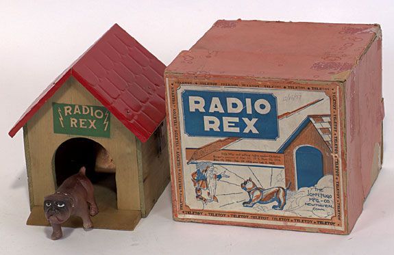
2      C HAPTER 26       •   AUTOMATIC S PEECH R ECOGNITION AND T EXT- TO -S PEECH

                     the Empress Maria Theresa the famous Mechanical Turk, a chess-playing automaton
                     consisting of a wooden box filled with gears, behind which sat a robot mannequin
                     who played chess by moving pieces with his mechanical arm. The Turk toured Eu-
                     rope and the Americas for decades, defeating Napoleon Bonaparte and even playing
                     Charles Babbage. The Mechanical Turk might have been one of the early successes
                     of artificial intelligence were it not for the fact that it was, alas, a hoax, powered by
                     a human chess player hidden inside the box.
                         What is less well known is that von Kempelen, an extraordinarily
                     prolific inventor, also built between
                     1769 and 1790 what was definitely
                     not a hoax: the first full-sentence
                     speech synthesizer, shown partially to
                     the right. His device consisted of a
                     bellows to simulate the lungs, a rub-
                     ber mouthpiece and a nose aperture, a
                     reed to simulate the vocal folds, var-
                     ious whistles for the fricatives, and a
                     small auxiliary bellows to provide the puff of air for plosives. By moving levers
                     with both hands to open and close apertures, and adjusting the flexible leather “vo-
                     cal tract”, an operator could produce different consonants and vowels.
                         More than two centuries later, we no longer build our synthesizers out of wood
            speech
         synthesis   and leather, nor do we need human operators. The modern task of speech synthesis,
    text-to-speech   also called text-to-speech or TTS, is exactly the reverse of ASR; to map text:
             TTS
                                                   It’s time for lunch!
                     to an acoustic waveform:

                         Modern speech synthesis has a wide variety of applications. TTS is used in
                     conversational agents that conduct dialogues with people, plays a role in devices
                     that read out loud for the blind or in games, and can be used to speak for sufferers
                     of neurological disorders, such as the late astrophysicist Steven Hawking who, after
                     he lost the use of his voice because of ALS, spoke by manipulating a TTS system.
                         In the next sections we’ll show how to do ASR with encoder-decoders, intro-
                     duce the CTC loss functions, the standard word error rate evaluation metric, and
                     describe how acoustic features are extracted. We’ll then see how TTS can be mod-
                     eled with almost the same algorithm in reverse, and conclude with a brief mention
                     of other speech tasks.

26.1             The Automatic Speech Recognition Task
                     Before describing algorithms for ASR, let’s talk about how the task itself varies.
                     One dimension of variation is vocabulary size. Some ASR tasks can be solved with
                     extremely high accuracy, like those with a 2-word vocabulary (yes versus no) or
            digit
      recognition    an 11 word vocabulary like digit recognition (recognizing sequences of digits in-
                     cluding zero to nine plus oh). Open-ended tasks like transcribing videos or human
                     conversations, with large vocabularies of up to 60,000 words, are much harder.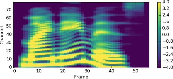
26.1   •   T HE AUTOMATIC S PEECH R ECOGNITION TASK              3

                      A second dimension of variation is who the speaker is talking to. Humans speak-
                 ing to machines (either dictating or talking to a dialogue system) are easier to recog-
  read speech    nize than humans speaking to humans. Read speech, in which humans are reading
                 out loud, for example in audio books, is also relatively easy to recognize. Recog-
conversational
       speech    nizing the speech of two humans talking to each other in conversational speech,
                 for example, for transcribing a business meeting, is the hardest. It seems that when
                 humans talk to machines, or read without an audience present, they simplify their
                 speech quite a bit, talking more slowly and more clearly.
                      A third dimension of variation is channel and noise. Speech is easier to recognize
                 if its recorded in a quiet room with head-mounted microphones than if it’s recorded
                 by a distant microphone on a noisy city street, or in a car with the window open.
                      A final dimension of variation is accent or speaker-class characteristics. Speech
                 is easier to recognize if the speaker is speaking the same dialect or variety that the
                 system was trained on. Speech by speakers of regional or ethnic dialects, or speech
                 by children can be quite difficult to recognize if the system is only trained on speak-
                 ers of standard dialects, or only adult speakers.
                      A number of publicly available corpora with human-created transcripts are used
                 to create ASR test and training sets to explore this variation; we mention a few of
  LibriSpeech    them here since you will encounter them in the literature. LibriSpeech is a large
                 open-source read-speech 16 kHz dataset with over 1000 hours of audio books from
                 the LibriVox project, with transcripts aligned at the sentence level (Panayotov et al.,
                 2015). It is divided into an easier (“clean”) and a more difficult portion (“other”)
                 with the clean portion of higher recording quality and with accents closer to US
                 English. This was done by running a speech recognizer (trained on read speech from
                 the Wall Street Journal) on all the audio, computing the WER for each speaker based
                 on the gold transcripts, and dividing the speakers roughly in half, with recordings
                 from lower-WER speakers called “clean” and recordings from higher-WER speakers
                 “other”.
 Switchboard          The Switchboard corpus of prompted telephone conversations between strangers
                 was collected in the early 1990s; it contains 2430 conversations averaging 6 min-
                 utes each, totaling 240 hours of 8 kHz speech and about 3 million words (Godfrey
                 et al., 1992). Switchboard has the singular advantage of an enormous amount of
                 auxiliary hand-done linguistic labeling, including parses, dialogue act tags, phonetic
CALLHOME         and prosodic labeling, and discourse and information structure. The CALLHOME
                 corpus was collected in the late 1990s and consists of 120 unscripted 30-minute
                 telephone conversations between native speakers of English who were usually close
                 friends or family (Canavan et al., 1997).
                      The Santa Barbara Corpus of Spoken American English (Du Bois et al., 2005) is
                 a large corpus of naturally occurring everyday spoken interactions from all over the
                 United States, mostly face-to-face conversation, but also town-hall meetings, food
                 preparation, on-the-job talk, and classroom lectures. The corpus was anonymized by
                 removing personal names and other identifying information (replaced by pseudonyms
                 in the transcripts, and masked in the audio).
    CORAAL            CORAAL is a collection of over 150 sociolinguistic interviews with African
                 American speakers, with the goal of studying African American Language (AAL),
                 the many variations of language used in African American communities (Kendall
                 and Farrington, 2020). The interviews are anonymized with transcripts aligned at
      CHiME      the utterance level. The CHiME Challenge is a series of difficult shared tasks with
                 corpora that deal with robustness in ASR. The CHiME 5 task, for example, is ASR of
                 conversational speech in real home environments (specifically dinner parties). The
4 C HAPTER 26 • AUTOMATIC S PEECH R ECOGNITION AND T EXT- TO -S PEECH
corpus contains recordings of twenty different dinner parties in real homes, each
with four participants, and in three locations (kitchen, dining area, living room),
recorded both with distant room microphones and with body-worn mikes. The
HKUST HKUST Mandarin Telephone Speech corpus has 1206 ten-minute telephone con-
versations between speakers of Mandarin across China, including transcripts of the
conversations, which are between either friends or strangers (Liu et al., 2006). The
AISHELL-1 AISHELL-1 corpus contains 170 hours of Mandarin read speech of sentences taken
from various domains, read by different speakers mainly from northern China (Bu
et al., 2017).
Figure 26.1 shows the rough percentage of incorrect words (the word error rate,
or WER, defined on page 15) from state-of-the-art systems on some of these tasks.
Note that the error rate on read speech (like the LibriSpeech audiobook corpus) is
around 2%; this is a solved task, although these numbers come from systems that re-
quire enormous computational resources. By contrast, the error rate for transcribing
conversations between humans is much higher; 5.8 to 11% for the Switchboard and
CALLHOME corpora. The error rate is higher yet again for speakers of varieties
like African American Vernacular English, and yet again for difficult conversational
tasks like transcription of 4-speaker dinner party speech, which can have error rates
as high as 81.3%. Character error rates (CER) are also much lower for read Man-
darin speech than for natural conversation.
English Tasks WER%
LibriSpeech audiobooks 960hour clean 1.4
LibriSpeech audiobooks 960hour other 2.6
Switchboard telephone conversations between strangers 5.8
CALLHOME telephone conversations between family 11.0
Sociolinguistic interviews, CORAAL (AAL) 27.0
CHiMe5 dinner parties with body-worn microphones 47.9
CHiMe5 dinner parties with distant microphones 81.3
Chinese (Mandarin) Tasks CER%
AISHELL-1 Mandarin read speech corpus 6.7
HKUST Mandarin Chinese telephone conversations 23.5
Figure 26.1 Rough Word Error Rates (WER = % of words misrecognized) reported around
2020 for ASR on various American English recognition tasks, and character error rates (CER)
for two Chinese recognition tasks.
26.2 Feature Extraction for ASR: Log Mel Spectrum
The first step in ASR is to transform the input waveform into a sequence of acoustic
feature vector feature vectors, each vector representing the information in a small time window
of the signal. Let’s see how to convert a raw wavefile to the most commonly used
features, sequences of log mel spectrum vectors. A speech signal processing course
is recommended for more details.
26.2.1 Sampling and Quantization
Recall from Section ?? that the first step is to convert the analog representations (first
air pressure and then analog electric signals in a microphone) into a digital signal.26.2 • F EATURE E XTRACTION FOR ASR: L OG M EL S PECTRUM 5
sampling This analog-to-digital conversion has two steps: sampling and quantization. A
sampling rate signal is sampled by measuring its amplitude at a particular time; the sampling rate
is the number of samples taken per second. To accurately measure a wave, we must
have at least two samples in each cycle: one measuring the positive part of the wave
and one measuring the negative part. More than two samples per cycle increases
the amplitude accuracy, but less than two samples will cause the frequency of the
wave to be completely missed. Thus, the maximum frequency wave that can be
measured is one whose frequency is half the sample rate (since every cycle needs
two samples). This maximum frequency for a given sampling rate is called the
Nyquist
frequency Nyquist frequency. Most information in human speech is in frequencies below
10,000 Hz, so a 20,000 Hz sampling rate would be necessary for complete accuracy.
But telephone speech is filtered by the switching network, and only frequencies less
than 4,000 Hz are transmitted by telephones. Thus, an 8,000 Hz sampling rate is
telephone- sufficient for telephone-bandwidth speech, and 16,000 Hz for microphone speech.
bandwidth
Although using higher sampling rates produces higher ASR accuracy, we can’t
combine different sampling rates for training and testing ASR systems. Thus if
we are testing on a telephone corpus like Switchboard (8 KHz sampling), we must
downsample our training corpus to 8 KHz. Similarly, if we are training on mul-
tiple corpora and one of them includes telephone speech, we downsample all the
wideband corpora to 8Khz.
Amplitude measurements are stored as integers, either 8 bit (values from -128–
127) or 16 bit (values from -32768–32767). This process of representing real-valued
quantization numbers as integers is called quantization; all values that are closer together than
the minimum granularity (the quantum size) are represented identically. We refer to
each sample at time index n in the digitized, quantized waveform as x[n].
26.2.2 Windowing
From the digitized, quantized representation of the waveform, we need to extract
spectral features from a small window of speech that characterizes part of a par-
ticular phoneme. Inside this small window, we can roughly think of the signal as
stationary stationary (that is, its statistical properties are constant within this region). (By
non-stationary contrast, in general, speech is a non-stationary signal, meaning that its statistical
properties are not constant over time). We extract this roughly stationary portion of
speech by using a window which is non-zero inside a region and zero elsewhere, run-
ning this window across the speech signal and multiplying it by the input waveform
to produce a windowed waveform.
frame The speech extracted from each window is called a frame. The windowing is
characterized by three parameters: the window size or frame size of the window
stride (its width in milliseconds), the frame stride, (also called shift or offset) between
successive windows, and the shape of the window.
To extract the signal we multiply the value of the signal at time n, s[n] by the
value of the window at time n, w[n]:
y[n] = w[n]s[n] (26.1)
rectangular The window shape sketched in Fig. 26.2 is rectangular; you can see the ex-
tracted windowed signal looks just like the original signal. The rectangular window,
however, abruptly cuts off the signal at its boundaries, which creates problems when
we do Fourier analysis. For this reason, for acoustic feature creation we more com-
Hamming monly use the Hamming window, which shrinks the values of the signal toward6 C HAPTER 26 • AUTOMATIC S PEECH R ECOGNITION AND T EXT- TO -S PEECH
Window
25 ms
Shift
10 Window
ms 25 ms
Shift
10 Window
ms 25 ms
Figure 26.2 Windowing, showing a 25 ms rectangular window with a 10ms stride.
zero at the window boundaries, avoiding discontinuities. Figure 26.3 shows both;
the equations are as follows (assuming a window that is L frames long):
1 0 ≤ n ≤ L−1
rectangular w[n] = (26.2)
0 otherwise
0.54 − 0.46 cos( 2πn 0 ≤ n ≤ L−1
Hamming w[n] = L ) (26.3)
0 otherwise
0.4999
0
–0.5
0 0.0475896
Time (s)
Rectangular window Hamming window
0.4999 0.4999
0 0
–0.5 –0.4826
0.00455938 0.0256563 0.00455938 0.0256563
Time (s) Time (s)
Figure 26.3 Windowing a sine wave with the rectangular or Hamming windows.
26.2.3 Discrete Fourier Transform
The next step is to extract spectral information for our windowed signal; we need to
know how much energy the signal contains at different frequency bands. The tool
for extracting spectral information for discrete frequency bands for a discrete-time
Discrete
Fourier (sampled) signal is the discrete Fourier transform or DFT.
transform
DFT26.2 • F EATURE E XTRACTION FOR ASR: L OG M EL S PECTRUM 7
The input to the DFT is a windowed signal x[n]...x[m], and the output, for each of
N discrete frequency bands, is a complex number X[k] representing the magnitude
and phase of that frequency component in the original signal. If we plot the mag-
nitude against the frequency, we can visualize the spectrum that we introduced in
Chapter 25. For example, Fig. 26.4 shows a 25 ms Hamming-windowed portion of
a signal and its spectrum as computed by a DFT (with some additional smoothing).
0.04414
Sound pressure level (dB/Hz)
20
0 0
–20
–0.04121
0.0141752 0.039295 0 8000
Time (s) Frequency (Hz)
(a) (b)
Figure 26.4 (a) A 25 ms Hamming-windowed portion of a signal from the vowel [iy]
and (b) its spectrum computed by a DFT.
We do not introduce the mathematical details of the DFT here, except to note
Euler’s formula that Fourier analysis relies on Euler’s formula, with j as the imaginary unit:
e jθ = cos θ + j sin θ (26.4)
As a brief reminder for those students who have already studied signal processing,
the DFT is defined as follows:
N−1
2π
x[n]e− j N kn
X
X[k] = (26.5)
n=0
fast Fourier A commonly used algorithm for computing the DFT is the fast Fourier transform
transform
FFT or FFT. This implementation of the DFT is very efficient but only works for values
of N that are powers of 2.
26.2.4 Mel Filter Bank and Log
The results of the FFT tell us the energy at each frequency band. Human hearing,
however, is not equally sensitive at all frequency bands; it is less sensitive at higher
frequencies. This bias toward low frequencies helps human recognition, since infor-
mation in low frequencies like formants is crucial for distinguishing values or nasals,
while information in high frequencies like stop bursts or fricative noise is less cru-
cial for successful recognition. Modeling this human perceptual property improves
speech recognition performance in the same way.
We implement this intuition by by collecting energies, not equally at each fre-
quency band, but according to the mel scale, an auditory frequency scale (Chap-
mel ter 25). A mel (Stevens et al. 1937, Stevens and Volkmann 1940) is a unit of pitch.
Pairs of sounds that are perceptually equidistant in pitch are separated by an equal
number of mels. The mel frequency m can be computed from the raw acoustic fre-
quency by a log transformation:
f
mel( f ) = 1127 ln(1 + ) (26.6)
7008 C HAPTER 26 • AUTOMATIC S PEECH R ECOGNITION AND T EXT- TO -S PEECH
We implement this intuition by creating a bank of filters that collect energy from
each frequency band, spread logarithmically so that we have very fine resolution
at low frequencies, and less resolution at high frequencies. Figure 26.5 shows a
sample bank of triangular filters that implement this idea, that can be multiplied by
the spectrum to get a mel spectrum.
1
Amplitude
0.5
0
0 7700
8K
Frequency (Hz)
mel spectrum m1 m2 ... mM
Figure 26.5 The mel filter bank (Davis and Mermelstein, 1980). Each triangular filter,
spaced logarithmically along the mel scale, collects energy from a given frequency range.
Finally, we take the log of each of the mel spectrum values. The human response
to signal level is logarithmic (like the human response to frequency). Humans are
less sensitive to slight differences in amplitude at high amplitudes than at low ampli-
tudes. In addition, using a log makes the feature estimates less sensitive to variations
in input such as power variations due to the speaker’s mouth moving closer or further
from the microphone.
26.3 Speech Recognition Architecture
The basic architecture for ASR is the encoder-decoder (implemented with either
RNNs or Transformers), exactly the same architecture introduced for MT in Chap-
ter 10. Generally we start from the log mel spectral features described in the previous
section, and map to letters, although it’s also possible to map to induced morpheme-
like chunks like wordpieces or BPE.
Fig. 26.6 sketches the standard encoder-decoder architecture, which is com-
AED monly referred to as the attention-based encoder decoder or AED, or listen attend
listen attend
and spell and spell (LAS) after the two papers which first applied it to speech (Chorowski
et al. 2014, Chan et al. 2016). The input is a sequence of t acoustic feature vectors
F = f1 , f2 , ..., ft , one vector per 10 ms frame. The output can be letters or word-
pieces; we’ll assume letters here. Thus the output sequence Y = (hSOSi, y1 , ..., ym hEOSi),
assuming special start of sequence and end of sequence tokens hsosi and heosi. and
each yi is a character; for English we might choose the set:
yi ∈ {a, b, c, ..., z, 0, ..., 9, hspacei, hcommai, hperiodi, hapostrophei, hunki}
Of course the encoder-decoder architecture is particularly appropriate when in-
put and output sequences have stark length differences, as they do for speech, with
very long acoustic feature sequences mapping to much shorter sequences of letters
or words. A single word might be 5 letters long but, supposing it lasts about 2
seconds, would take 200 acoustic frames (of 10ms each).
Because this length difference is so extreme for speech, encoder-decoder ar-
chitectures for speech need to have a special compression stage that shortens the
acoustic feature sequence before the encoder stage. (Alternatively, we can use a loss26.3 • S PEECH R ECOGNITION A RCHITECTURE 9
y1 y2 y3 y4 y5 y6 y7 y8 y9 ym
i t ‘ s t i m e …
H
DECODER
ENCODER
x1 xn
i t ‘ s t i m …
Shorter sequence X …
Subsampling
80-dimensional
log Mel spectrum f1 … ft
per frame
Feature Computation
Figure 26.6 Schematic architecture for an encoder-decoder speech recognizer.
function that is designed to deal well with compression, like the CTC loss function
we’ll introduce in the next section.)
The goal of the subsampling is to produce a shorter sequence X = x1 , ..., xn that
will be the input to the encoder. The simplest algorithm is a method sometimes
low frame rate called low frame rate (Pundak and Sainath, 2016): for time i we stack (concatenate)
the acoustic feature vector fi with the prior two vectors fi−1 and fi−2 to make a new
vector three times longer. Then we simply delete fi−1 and fi−2 . Thus instead of
(say) a 40-dimensional acoustic feature vector every 10 ms, we have a longer vector
(say 120-dimensional) every 30 ms, with a shorter sequence length n = 3t .1
After this compression stage, encoder-decoders for speech use the same archi-
tecture as for MT or other text, composed of either RNNs (LSTMs) or Transformers.
For inference, the probability of the output string Y is decomposed as:
n
Y
p(y1 , . . . , yn ) = p(yi |y1 , . . . , yi−1 , X) (26.7)
i=1
We can produce each letter of the output via greedy decoding:
ŷi = argmaxchar∈ Alphabet P(char|y1 ...yi−1 , X) (26.8)
Alternatively we can use beam search as described in the next section. this is partic-
ularly relevant when we are adding a language model.
Adding a language model Since an encoder-decoder model is essentially a con-
ditional language model, encoder-decoders implicitly learn a language model for the
output domain of letters from their training data. However, the training data (speech
paired with text transcriptions) may not include sufficient text to train a good lan-
guage model. After all, it’s easier to find enormous amounts of pure text training
data than it is to find text paired with speech. Thus we can can usually improve a
model at least slightly by incorporating a very large language model.
The simplest way to do this is to use beam search to get a final beam of hy-
n-best list pothesized sentences; this beam is sometimes called an n-best list. We then use a
rescore language model to rescore each hypothesis on the beam. The scoring is doing by in-
1 There are also more complex alternatives for subsampling, like using a convolutional net that down-
samples with max pooling, or layers of pyramidal RNNs, RNNs where each successive layer has half
the number of RNNs as the previous layer.10 C HAPTER 26 • AUTOMATIC S PEECH R ECOGNITION AND T EXT- TO -S PEECH
terpolating the score assigned by the language model with the encoder-decoder score
used to create the beam, with a weight λ tuned on a held-out set. Also, since most
models prefer shorter sentences, ASR systems normally have some way of adding a
length factor. One way to do this is to normalize the probability by the number of
characters in the hypothesis |Y |c . The following is thus a typical scoring function
(Chan et al., 2016):
1
score(Y |X) = log P(Y |X) + λ log PLM (Y ) (26.9)
|Y |c
26.3.1 Learning
Encoder-decoders for speech are trained with the normal cross-entropy loss gener-
ally used for conditional language models. At timestep i of decoding, the loss is the
log probability of the correct token (letter) yi :
LCE = − log p(yi |y1 , . . . , yi−1 , X) (26.10)
The loss for the entire sentence is the sum of these losses:
m
X
LCE = − log p(yi |y1 , . . . , yi−1 , X) (26.11)
i=1
This loss is then backpropagated through the entire end-to-end model to train the
entire encoder-decoder.
As we described in Chapter 10, we normally use teacher forcing, in which the
decoder history is forced to be the correct gold yi rather than the predicted ŷi . It’s
also possible to use a mixture of the gold and decoder output, for example using
the gold output 90% of the time, but with probability .1 taking the decoder output
instead:
LCE = − log p(yi |y1 , . . . , ŷi−1 , X) (26.12)
26.4 CTC
We pointed out in the previous section that speech recognition has two particular
properties that make it very appropriate for the encoder-decoder architecture, where
the encoder produces an encoding of the input that the decoder uses attention to
explore. First, in speech we have a very long acoustic input sequence X mapping to
a much shorter sequence of letters Y , and second, it’s hard to know exactly which
part of X maps to which part of Y .
In this section we briefly introduce an alternative to encoder-decoder: an algo-
CTC rithm and loss function called CTC, short for Connectionist Temporal Classifica-
tion (Graves et al., 2006), that deals with these problems in a very different way. The
intuition of CTC is to output a single character for every frame of the input, so that
the output is the same length as the input, and then to apply a collapsing function
that combines sequences of identical letters, resulting in a shorter sequence.
Let’s imagine inference on someone saying the word dinner, and let’s suppose
we had a function that chooses the most probable letter for each input spectral frame
representation xi . We’ll call the sequence of letters corresponding to each input26.4 • CTC 11
alignment frame an alignment, because it tells us where in the acoustic signal each letter aligns
to. Fig. 26.7 shows one such alignment, and what happens if we use a collapsing
function that just removes consecutive duplicate letters.
Y (ouput) d i n e r
A (alignment) d i i n n n n e r r r r r r
X (input) x1 x2 x3 x4 x5 x6 x7 x8 x9 x10 x11 x12 x13 x14
wavefile
Figure 26.7 A naive algorithm for collapsinging an alignment between input and letters.
Well, that doesn’t work; our naive algorithm has transcribed the speech as diner,
not dinner! Collapsing doesn’t handle double letters. There’s also another problem
with our naive function; it doesn’t tell us what symbol to align with silence in the
input. We don’t want to be transcribing silence as random letters!
The CTC algorithm solves both problems by adding to the transcription alphabet
blank a special symbol for a blank, which we’ll represent as . The blank can be used in
the alignment whenever we don’t want to transcribe a letter. Blank can also be used
between letters; since our collapsing function collapses only consecutive duplicate
letters, it won’t collapse across . More formally, let’s define the mapping B : a → y
between an alignment a and an output y, which collapses all repeated letters and
then removes all blanks. Fig. 26.8 sketches this collapsing function B.
Y (output) d i n n e r
remove blanks d i n n e r
merge duplicates d i ␣ n ␣ n e r ␣
A (alignment) d i ␣ n n ␣ n e r r r r ␣ ␣
X (input) x1 x2 x3 x4 x5 x6 x7 x8 x9 x10 x11 x12 x13 x14
Figure 26.8 The CTC collapsing function B, showing the space blank character ; repeated
(consecutive) characters in an alignment A are removed to form the output Y .
The CTC collapsing function is many-to-one; lots of different alignments map to
the same output string. For example, the alignment shown in Fig. 26.8 is not the only
alignment that results in the string dinner. Fig. 26.9 shows some other alignments
that would produce the same output.
d i i n ␣ n n e e e r r ␣ r
d d i n n ␣ n e r r ␣ ␣ ␣ ␣
d d d i n ␣ n n ␣ ␣ ␣ e r r
Figure 26.9 Three other legimate alignments producing the transcript dinner.
It’s useful to think of the set of all alignments that might produce the same output12 C HAPTER 26 • AUTOMATIC S PEECH R ECOGNITION AND T EXT- TO -S PEECH
Y . We’ll use the inverse of our B function, called B−1 , and represent that set as
B−1 (Y ).
26.4.1 CTC Inference
Before we see how to compute PCTC (Y |X) let’s first see how CTC assigns a proba-
bility to one particular alignment  = {â1 , . . . , ân }. CTC makes a strong conditional
independence assumption: it assumes that, given the input X, the CTC model output
at at time t is independent of the output labels at any other time ai . Thus:
T
Y
PCTC (A|X) = p(at |X) (26.13)
t=1
Thus to find the best alignment  = {â1 , . . . , âT } we can greedily choose the charac-
ter with the max probability at each time step t:
ât = argmax pt (c|X) (26.14)
c∈C
We then pass the resulting sequence A to the CTC collapsing function B to get the
output sequence Y .
Let’s talk about how this simple inference algorithm for finding the best align-
ment A would be implemented. Because we are making a decision at each time
point, we can treat CTC as a sequence-modeling task, where we output one letter
ŷt at time t corresponding to each input token xt , eliminating the need for a full de-
coder. Fig. 26.10 sketches this architecture, where we take an encoder, produce a
hidden state ht at each timestep, and decode by taking a softmax over the character
vocabulary at each time step.
output letter y1 y2 y3 y4 y5 … yn
sequence Y
i i i t t …
Classifier …
+softmax
ENCODER
Shorter input
sequence X x1 … xn
Subsampling
log Mel spectrum f1 … ft
Feature Computation
Figure 26.10 Inference with CTC: using an encoder-only model, with decoding done by
simple softmaxes over the hidden state ht at each output step.
Alas, there is a potential flaw with the inference algorithm sketched in (Eq. 26.14)
and Fig. 26.9. The problem is that we chose the most likely alignment A, but the
most likely alignment may not correspond to the most likely final collapsed output
string Y . That’s because there are many possible alignments that lead to the same
output string, and hence the most likely output string might correspond to the most26.4 • CTC 13
probable alignment. For example, imagine the most probable alignment A for an
input X = [x1 x2 x3 ] is the string [a b ] but the next two most probable alignments are
[b b] and [ b b]. The output Y =[b b], summing over those two alignments, might
be more probable than Y =[a b].
For this reason, the most probable output sequence Y is the one that has, not
the single best CTC alignment, but the highest sum over the probability of all its
possible alignments:
X
PCTC (Y |X) = P(A|X)
A∈B−1 (Y )
X T
Y
= p(at |ht )
A∈B−1 (Y ) t=1
Ŷ = argmax PCTC (Y |X) (26.15)
Y
Alas, summing over all alignments is very expensive (there are a lot of alignments),
so we approximate this sum by using a version of Viterbi beam search that cleverly
keeps in the beam the high-probability alignments that map to the same output string,
and sums those as an approximation of (Eq. 26.15). See Hannun (2017) for a clear
explanation of this extension of beam search for CTC.
Because of the strong conditional independence assumption mentioned earlier
(that the output at time t is independent of the output at time t − 1, given the input),
CTC does not implicitly learn a language model over the data (unlike the attention-
based encoder-decoder architectures). It is therefore essential when using CTC to
interpolate a language model (and some sort of length factor L(Y )) using interpola-
tion weights that are trained on a dev set:
scoreCTC (Y |X) = log PCTC (Y |X) + λ1 log PLM (Y )λ2 L(Y ) (26.16)
26.4.2 CTC Training
To train a CTC-based ASR system, we use negative log-likelihood loss with a special
CTC loss function. Thus the loss for an entire dataset D is the sum of the negative
log-likelihoods of the correct output Y for each input X:
X
LCTC = − log PCTC (Y |X) (26.17)
(X,Y )∈D
To compute CTC loss function for a single input pair (X,Y ), we need the probability
of the output Y given the input X. As we saw in Eq. 26.15, to compute the probability
of a given output Y we need to sum over all the possible alignments that would
collapse to Y . In other words:
X T
Y
PCTC (Y |X) = p(at |ht ) (26.18)
A∈B−1 (Y ) t=1
Naively summing over all possible alignments in not feasible (there are too many
alignments). However, we can efficiently compute the sum by using dynamic pro-
gramming to merge alignments, with a version of the forward-backward algo-
rithm also used to train HMMs (Appendix A) and CRFs. The original dynamic pro-
gramming algorithms for both training and inference are laid out in (Graves et al.,
2006); see (Hannun, 2017) for a detailed explanation of both.14 C HAPTER 26 • AUTOMATIC S PEECH R ECOGNITION AND T EXT- TO -S PEECH
26.4.3 Combining CTC and Encoder-Decoder
It’s also possible to combine the two architectures/loss functions we’ve described,
the cross-entropy loss from the encoder-decoder architecture, and the CTC loss.
Fig. 26.11 shows a sketch. For training, we can can simply weight the two losses
with a λ tuned on a dev set:
L = −λ log Pencdec (Y |X) − (1 − λ ) log Pctc (Y |X) (26.19)
For inference, we can combine the two with the language model (or the length
penalty), again with learned weights:
Ŷ = argmax [λ log Pencdec (Y |X) − (1 − λ ) log PCTC (Y |X) + γ log PLM (Y )] (26.20)
Y
i t ’ s t i m e …
CTC Loss Encoder-Decoder Loss
…
DECODER
… H
ENCODER
i t ‘ s t i m …
…
x1 xn
Figure 26.11 Combining the CTC and encoder-decoder loss functions.
26.4.4 Streaming Models: RNN-T for improving CTC
Because of the strong independence assumption in CTC (assuming that the output
at time t is independent of the output at time t − 1), recognizers based on CTC
don’t achieve as high an accuracy as the attention-based encoder-decoder recog-
nizers. CTC recognizers have the advantage, however, that they can be used for
streaming streaming. Streaming means recognizing words on-line rather than waiting until
the end of the sentence to recognize them. Streaming is crucial for many applica-
tions, from commands to dictation, where we want to start recognition while the
user is still talking. Algorithms that use attention need to compute the hidden state
sequence over the entire input first in order to provide the attention distribution con-
text, before the decoder can start decoding. By contrast, a CTC algorithm can input
letters from left to right immediately.
If we want to do streaming, we need a way to improve CTC recognition to re-
move the conditional independent assumption, enabling it to know about output his-
RNN-T tory. The RNN-Transducer (RNN-T), shown in Fig. 26.12, is just such a model
(Graves 2012, Graves et al. 2013). The RNN-T has two main components: a CTC
acoustic model, and a separate language model component called the predictor that
conditions on the output token history. At each time step t, the CTC encoder outputs
a hidden state htenc given the input x1 ...xt . The language model predictor takes as in-
pred
put the previous output token (not counting blanks), outputting a hidden state hu .
The two are passed through another network whose output is then passed through a26.5 • ASR E VALUATION : W ORD E RROR R ATE 15
softmax to predict the next character.
X
PRNN−T (Y |X) = P(A|X)
A∈B−1 (Y )
X T
Y
= p(at |ht , y16 C HAPTER 26 • AUTOMATIC S PEECH R ECOGNITION AND T EXT- TO -S PEECH
2005). Sclite is given a series of reference (hand-transcribed, gold-standard) sen-
tences and a matching set of hypothesis sentences. Besides performing alignments,
and computing word error rate, sclite performs a number of other useful tasks. For
example, for error analysis it gives useful information such as confusion matrices
showing which words are often misrecognized for others, and summarizes statistics
of words that are often inserted or deleted. sclite also gives error rates by speaker
(if sentences are labeled for speaker ID), as well as useful statistics like the sentence
Sentence error error rate, the percentage of sentences with at least one word error.
rate
Statistical significance for ASR: MAPSSWE or MacNemar
As with other language processing algorithms, we need to know whether a particular
improvement in word error rate is significant or not.
The standard statistical tests for determining if two word error rates are different
is the Matched-Pair Sentence Segment Word Error (MAPSSWE) test, introduced in
Gillick and Cox (1989).
The MAPSSWE test is a parametric test that looks at the difference between
the number of word errors the two systems produce, averaged across a number of
segments. The segments may be quite short or as long as an entire utterance; in
general, we want to have the largest number of (short) segments in order to justify
the normality assumption and to maximize power. The test requires that the errors
in one segment be statistically independent of the errors in another segment. Since
ASR systems tend to use trigram LMs, we can approximate this requirement by
defining a segment as a region bounded on both sides by words that both recognizers
get correct (or by turn/utterance boundaries). Here’s an example from NIST (2007)
with four regions:
I II III IV
REF: |it was|the best|of|times it|was the worst|of times| |it was
| | | | | | | |
SYS A:|ITS |the best|of|times it|IS the worst |of times|OR|it was
| | | | | | | |
SYS B:|it was|the best| |times it|WON the TEST |of times| |it was
In region I, system A has two errors (a deletion and an insertion) and system B
has zero; in region III, system A has one error (a substitution) and system B has two.
Let’s define a sequence of variables Z representing the difference between the errors
in the two systems as follows:
NAi the number of errors made on segment i by system A
NBi the number of errors made on segment i by system B
Z NAi − NBi , i = 1, 2, · · · , n where n is the number of segments
In the example above, the sequence of Z values is {2, −1, −1, 1}. Intuitively, if
the two systems are identical, we would expect the average difference, that is, the
average of the Z values, to be zero. If we call the true average of the differences
muz , we would thus like to know whether muz = 0. Following closely the original
proposal and notation of Gillick P
and Cox (1989), we can estimate the true average
from our limited sample as µ̂z = ni=1 Zi /n. The estimate of the variance of the Zi ’s
is
n
1 X
σz2 = (Zi − µz )2 (26.21)
n−1
i=126.6 • TTS 17
Let
µ̂z
W= √ (26.22)
σz / n
For a large enough n (> 50), W will approximately have a normal distribution with
unit variance. The null hypothesis is H0 : µz = 0, and it can thus be rejected if
2 ∗ P(Z ≥ |w|) ≤ 0.05 (two-tailed) or P(Z ≥ |w|) ≤ 0.05 (one-tailed), where Z is
standard normal and w is the realized value W ; these probabilities can be looked up
in the standard tables of the normal distribution.
McNemar’s test Earlier work sometimes used McNemar’s test for significance, but McNemar’s
is only applicable when the errors made by the system are independent, which is not
true in continuous speech recognition, where errors made on a word are extremely
dependent on errors made on neighboring words.
Could we improve on word error rate as a metric? It would be nice, for exam-
ple, to have something that didn’t give equal weight to every word, perhaps valuing
content words like Tuesday more than function words like a or of. While researchers
generally agree that this would be a good idea, it has proved difficult to agree on
a metric that works in every application of ASR. For dialogue systems, however,
where the desired semantic output is more clear, a metric called slot error rate or
concept error rate has proved extremely useful; it is discussed in Chapter 24 on page
??.
26.6 TTS
The goal of text-to-speech (TTS) systems is to map from strings of letters to wave-
forms, a technology that’s important for a variety of applications from dialogue sys-
tems to games to education.
Like ASR systems, TTS systems are generally based on the encoder-decoder
architecture, either using LSTMs or Transformers. There is a general difference in
training. The default condition for ASR systems is to be speaker-independent: they
are trained on large corpora with thousands of hours of speech from many speakers
because they must generalize well to an unseen test speaker. By contrast, in TTS, it’s
less crucial to use multiple voices, and so basic TTS systems are speaker-dependent:
trained to have a consistent voice, on much less data, but all from one speaker. For
example, one commonly used public domain dataset, the LJ speech corpus, consists
of 24 hours of one speaker, Linda Johnson, reading audio books in the LibriVox
project (Ito and Johnson, 2017), much smaller than standard ASR corpora which are
hundreds or thousands of hours.2
We generally break up the TTS task into two components. The first component
is an encoder-decoder model for spectrogram prediction: it maps from strings of
letters to mel spectrographs: sequences of mel spectral values over time. Thus we
2 There is also recent TTS research on the task of multi-speaker TTS, in which a system is trained on
speech from many speakers, and can switch between different voices.18 C HAPTER 26 • AUTOMATIC S PEECH R ECOGNITION AND T EXT- TO -S PEECH
might map from this string:
It’s time for lunch!
to the following mel spectrogram:
The second component maps from mel spectrograms to waveforms. Generating
vocoding waveforms from intermediate representations like spectrograms is called vocoding
vocoder and this second component is called a vocoder:
These standard encoder-decoder algorithms for TTS are still quite computation-
ally intensive, so a significant focus of modern research is on ways to speed them
up.
26.6.1 TTS Preprocessing: Text normalization
Before either of these two steps, however, TTS systems require text normaliza-
non-standard tion preprocessing for handling non-standard words: numbers, monetary amounts,
words
dates, and other concepts that are verbalized differently than they are spelled. A TTS
system seeing a number like 151 needs to know to verbalize it as one hundred fifty
one if it occurs as $151 but as one fifty one if it occurs in the context 151 Chapulte-
pec Ave.. The number 1750 can be spoken in at least four different ways, depending
on the context:
seventeen fifty: (in “The European economy in 1750”)
one seven five zero: (in “The password is 1750”)
seventeen hundred and fifty: (in “1750 dollars”)
one thousand, seven hundred, and fifty: (in “1750 dollars”)
Often the verbalization of a non-standard word depends on its meaning (what
Taylor (2009) calls its semiotic class). Fig. 26.13 lays out some English non-
standard word types.
Many classes have preferred realizations. A year is generally read as paired
digits (e.g., seventeen fifty for 1750). $3.2 billion must be read out with the
word dollars at the end, as three point two billion dollars, Some abbre-
viations like N.Y. are expanded (to New York), while other acronyms like GPU are
pronounced as letter sequences. In languages with grammatical gender, normal-
ization may depend on morphological properties. In French, the phrase 1 mangue
(‘one mangue’) is normalized to une mangue, but 1 ananas (‘one pineapple’) is
normalized to un ananas. In German, Heinrich IV (‘Henry IV’) can be normalized
to Heinrich der Vierte, Heinrich des Vierten, Heinrich dem Vierten, or
Heinrich den Vierten depending on the grammatical case of the noun (Demberg,
2006).26.6 • TTS 19
semiotic class examples verbalization
abbreviations gov’t, N.Y., mph government
acronyms read as letters GPU, D.C., PC, UN, IBM G P U
cardinal numbers 12, 45, 1/2, 0.6 twelve
ordinal numbers May 7, 3rd, Bill Gates III seventh
numbers read as digits Room 101 one oh one
times 3.20, 11:45 eleven forty five
dates 28/02 (or in US, 2/28) February twenty eighth
years 1999, 80s, 1900s, 2045 nineteen ninety nine
money $3.45, e250, $200K three dollars forty five
money in tr/m/billions $3.45 billion three point four five billion dollars
percentage 75% 3.4% seventy five percent
Figure 26.13 Some types of non-standard words in text normalization; see Sproat et al.
(2001) and (van Esch and Sproat, 2018) for many more.
Modern end-to-end TTS systems can learn to do some normalization themselves,
but TTS systems are only trained on a limited amount of data (like the 220,000 words
we mentioned above for the LJ corpus (Ito and Johnson, 2017)), and so a separate
normalization step is important.
Normalization can be done by rule or by an encoder-decoder model. Rule-based
normalization is done in two stages: tokenization and verbalization. In the tokeniza-
tion stage we hand-write write rules to detect non-standard words. These can be
regular expressions, like the following for detecting years:
/(1[89][0-9][0-9])|(20[0-9][0-9]/
A second pass of rules express how to verbalize each semiotic class. Larger TTS
systems instead use more complex rule-systems, like the Kestral system of (Ebden
and Sproat, 2015), which first classifies and parses each input into a normal form
and then produces text using a verbalization grammar. Rules have the advantage
that they don’t require training data, and they can be designed for high precision, but
can be brittle, and require expert rule-writers so are hard to maintain.
The alternative model is to use encoder-decoder models, which have been shown
to work better than rules for such transduction tasks, but do require expert-labeled
training sets in which non-standard words have been replaced with the appropriate
verbalization; such training sets for some languages are available (Sproat and Gor-
man 2018, Zhang et al. 2019).
In the simplest encoder-decoder setting, we simply treat the problem like ma-
chine translation, training a system to map from:
They live at 224 Mission St.
to
They live at two twenty four Mission Street
While encoder-decoder algorithms are highly accurate, they occasionally pro-
duce errors that are egregious; for example normalizing 45 minutes as forty five mil-
limeters. To address this, more complex systems use mechanisms like lightweight
covering grammars, which enumerate a large set of possible verbalizations but
don’t try to disambiguate, to constrain the decoding to avoid such outputs (Zhang
et al., 2019).
26.6.2 TTS: Spectrogram prediction
The exact same architecture we described for ASR—the encoder-decoder with attention–
can be used for the first component of TTS. Here we’ll give a simplified overview20 C HAPTER 26 • AUTOMATIC S PEECH R ECOGNITION AND T EXT- TO -S PEECH
Tacotron2 of the Tacotron2 architecture (Shen et al., 2018), which extends the earlier Tacotron
Wavenet (Wang et al., 2017) architecture and the Wavenet vocoder (van den Oord et al.,
2016). Fig. 26.14 sketches out the entire architecture.
The encoder’s job is to take a sequence of letters and produce a hidden repre-
sentation representing the letter sequence, which is then used by the attention mech-
anism in the decoder. The Tacotron2 encoder first maps every input grapheme to
a 512-dimensional character embedding. These are then passed through a stack
of 3 convolutional layers, each containing 512 filters with shape 5 × 1, i.e. each
filter spanning 5 characters, to model the larger letter context. The output of the
final convolutional layer is passed through a biLSTM to produce the final encod-
ing. It’s common to use a slightly higher quality (but slower) version of attention
location-based called location-based attention, in which the computation of the α values (Eq. ??
attention
in Chapter 10) makes use of the α values from the prior time-state.
In the decoder, the predicted mel spectrum from the prior time slot is passed
through a small pre-net as a bottleneck. This prior output is then concatenated with
the encoder’s attention vector context and passed through 2 LSTM layers. The out-
put of this LSTM is used in two ways. First, it is passed through a linear layer, and
some output processing, to autoregressively predict one 80-dimensional log-mel fil-
terbank vector frame (50 ms, with a 12.5 ms stride) at each step. Second, it is passed
through another linear layer to a sigmoid to make a “stop token prediction” decision
about whether to stop producing output.
While linear spectrograms discard phase information (and are
therefore lossy), algorithms such as Griffin-Lim [14] are capable of
estimating this discarded information, which enables time-domain Vocoder
conversion via the inverse short-time Fourier transform. Mel spectro-
grams discard even more information, presenting a challenging in-
verse problem. However, in comparison to the linguistic and acoustic
Decoder
features used in WaveNet, the mel spectrogram is a simpler, lower-
level acoustic representation of audio signals. It should therefore
be straightforward for a similar WaveNet model conditioned on mel
spectrograms to generate audio, essentially as a neural vocoder. In-
deed, we will show that it is possible to generate high quality audio
from mel spectrograms using a modified WaveNet architecture.
2.2. Spectrogram Prediction Network
Encoder
As in Tacotron, mel spectrograms are computed through a short-
time Fourier transform (STFT) using a 50 ms frame size, 12.5 ms
frame hop, and a Hann window function. We experimented with a
Figure 26.14
5 ms frame hop to match the frequency of the conditioning inputs The Tacotron2
Fig. 1. Blockarchitecture: An encoder-decoder
diagram of the Tacotron maps from graphemes to
2 system architecture.
mel spectrograms,
in the original WaveNet, but the corresponding increase in temporal followed by a vocoder that maps to wavefiles. Figure modified from Shen
resolution resulted in significantly more pronunciation issues.
et al. (2018). post-net layer is comprised of 512 filters with shape 5 ⇥ 1 with batch
We transform the STFT magnitude to the mel scale using an 80
channel mel filterbank spanning 125 Hz to 7.6 kHz, followed by log normalization, followed by tanh activations on all but the final layer.
dynamic range compression. Prior to log compression,The the filterbank We minimize the summed mean squared error (MSE) from before
system isand trained on gold log-mel filterbank features, using teacher forcing,
after the post-net to aid convergence. We also experimented
output magnitudes are clipped to a minimum value of 0.01 in order
to limit dynamic range in the logarithmic domain.that is the decoder is afed
with the correct
log-likelihood log-model
loss by modeling thespectral featurewith
output distribution at each decoder step
The network is composed of an encoder and ainstead
decoder withof atten- a Mixturedecoder
the predicted Density Network
output[23, 24] tothe
from avoid assuming
prior step.a constant
tion. The encoder converts a character sequence into a hidden feature variance over time, but found that these were more difficult to train
representation which the decoder consumes to predict a spectrogram. and they did not lead to better sounding samples.
Input characters are represented using a learned 512-dimensional In parallel to spectrogram frame prediction, the concatenation of
26.6.3 TTS: Vocoding
character embedding, which are passed through a stack of 3 convolu- decoder LSTM output and the attention context is projected down
tional layers each containing 512 filters with shape 5 ⇥ 1, i.e., where to a scalar and passed through a sigmoid activation to predict the
by batch The
WaveNet
each filter spans 5 characters, followed vocoder
normalization [18]for Tacotron 2 isthean
probability that adaptation
output sequence has the WaveNet
ofcompleted. This “stopvocoder
token” (van den Oord
and ReLU activations. As in Tacotron, these convolutional layers prediction is used during inference to allow the model to dynamically
et al., 2016).
model longer-term context (e.g., N -grams) in the input character
Here we’ll give a somewhat simplified description
determine when to terminate generation instead of always generating
of vocoding using
WaveNet.
sequence. The output of the final convolutional layer is passed into a for a fixed duration. Specifically, generation completes at the first
Recall
single bi-directional [19] LSTM [20] layer containing 512 that theframe
units (256 goalforofwhich
thethis probabilityprocess
vocoding exceeds a here
threshold
willof be
0.5. to invert a log mel spec-
in each direction) to generate the encoded features. The convolutional layers in the network are regularized using
The encoder output is consumed by an attentiontrum representations
network which dropoutback
[25] into a time-domain
with probability waveform
0.5, and LSTM layers arerepresentation.
regularized WaveNet is
an autoregressive
summarizes the full encoded sequence as a fixed-length context vector network,
using zoneout like theprobability
[26] with language 0.1.models
In order towe introduced
introduce output in Chapter 9. It
for each decoder output step. We use the location-sensitive attention variation at inference time, dropout with probability 0.5 is applied
from [21], which extends the additive attention mechanism [22] to only to layers in the pre-net of the autoregressive decoder.
use cumulative attention weights from previous decoder time steps In contrast to the original Tacotron, our model uses simpler build-
as an additional feature. This encourages the model to move forward ing blocks, using vanilla LSTM and convolutional layers in the en-
consistently through the input, mitigating potential failure modes coder and decoder instead of “CBHG” stacks and GRU recurrent
where some subsequences are repeated or ignored by the decoder. layers. We do not use a “reduction factor”, i.e., each decoder step
Attention probabilities are computed after projecting inputs and lo- corresponds to a single spectrogram frame.
cation features to 128-dimensional hidden representations. Location
features are computed using 32 1-D convolution filters of length 31.26.6 • TTS 21
takes spectrograms as input and produces audio output represented as sequences of
8-bit mu-law (page ??). The probability of a waveform , a sequence of 8-bit mu-law
values Y = y1 , ..., yt , given an intermediate input mel spectrogram h is computed as:
t
Because models with causal convolutions do tnot
|y1 ,have
..., yrecurrent connections, they are typically
(26.23) faster
Y
p(Y ) = P(y t−1 , h1 , ..., ht )
to train than RNNs, especially when applied t=1 to very long sequences. One of the problems of causal
convolutions is that they require many layers, or large filters to increase the receptive field. For
example, in Fig.probability
This 2 the receptive field is is
distribution only 5 (= #layers
modeled by a stack + filter length convolution
of special - 1). In this paper
layers,we use
dilatedwhich
convolutions
includetoaincrease
specificthe receptive field
convolutional by orders
structure of magnitude,
called without greatlyand
dilated convolutions, increasing
a
computational
specific cost.
non-linearity function.
A dilated convolution
A dilated convolution (also calledisà atrous,
subtype of causal with
or convolution convolutional
holes) is alayer. Causalwhere
convolution or the
filter ismasked
applied convolutions
over an area larger
look than
only itsat length
the past by input,
skipping inputthan
rather values
thewith a certain
future; the pre-step. It is
equivalent to a of
diction convolution
yt+1 can withonly adepend
larger filter
on yderived
1 , ..., yt ,from thefor
useful original filter by dilating
autoregressive it with zeros,
left-to-right
but is significantly
dilated processing. more
In efficient.
dilated A dilated convolution
convolutions, at each effectively
successive allows
layer we the network
apply the to operate on
convolu-
convolutions
a coarser scale
tional thanover
filter withaaspan
normal convolution.
longer This isby
than its length similar
skipping to pooling or strided
input values. convolutions,
Thus at time but
here the output has the same size as the input. As a special case, dilated convolution with dilation
1 yields t with a dilationconvolution.
the standard value of 1, aFig. convolutional
3 depicts dilatedfilter of length
causal 2 would seefor
convolutions input values1, 2, 4,
dilations
x and
and 8. Dilated
t x . But a filter with a distillation value of 2 would
convolutions have previously been used in various contexts, e.g. signal
t−1 skip an input, so would
processing
see input values
(Holschneider et al., 1989; xt and x .
Dutilleux,
t−1 Fig. 26.15 shows the computation of
1989), and image segmentation (Chen et al., 2015; the output at time Yu &
Koltun,t with
2016).4 dilated convolution layers with dilation values, 1, 2, 4, and 8.
Output
Dilation = 8
Hidden Layer
Dilation = 4
Hidden Layer
Dilation = 2
Hidden Layer
Dilation = 1
Input
Figure 26.15 Dilated convolutions, showing one dilation cycle size of 4, i.e., dilation values
of 1, 2, 4, 8. Figure from van den Oord et al. (2016).
Figure 3: Visualization of a stack of dilated causal convolutional layers.
Stacked dilatedThe Tacotron
convolutions2 synthesizer
enable networks uses 12 convolutional
to have very large layers
receptivein two
fieldscycles with
with just a lay-
a few
dilation
ers, while cycle size
preserving of 6,resolution
the input meaning that the firstthe
throughout 6 layers
network have dilations
as well of 1, 2, 4, 8,efficiency.
as computational 16,
In this and
paper, 32.the
anddilation
the nextis doubled
6 layersfor every
again layer
have up to a of
dilations limit
1, and
2, 4,then repeated:
8, 16, and 32.e.g.Dilated
convolutions allow1,the vocoder
2, 4, to 1,
. . . , 512, grow
2, 4,the
. . .receptive
, 512, 1, 2,field
4, . .exponentially
. , 512. with depth.
The intuition WaveNet predicts
behind this mu-law is
configuration audio samples.
two-fold. First, Recall from page
exponentially ?? that
increasing thethis is a factor
dilation
resultsstandard compression
in exponential receptive forfield
audio in which
growth with the
depthvalues
(Yu at& each
Koltun, sampling
2016). timestep
For exampleare each
1, 2, 4,compressed
. . . , 512 block into
has8-bits. Thisfield
receptive means that1024,
of size we can andpredict
can be the seenvalue of each
as a more sample
efficient and dis-
with (non-linear)
criminative a simple 256-way categorical
counterpart classifier.
of a 1⇥1024 The output
convolution. of thestacking
Second, dilated convolutions
these blocks further
increases the model
is thus passedcapacity
throughand the receptive
a softmax whichfield
makes size.this 256-way decision.
The spectrogram prediction encoder-decoder and the WaveNet vocoder are trained
2.2 Sseparately. After the spectrogram predictor is trained, the spectrogram prediction
OFTMAX DISTRIBUTIONS
network is run in teacher-forcing mode, with each predicted spectral frame condi-
One approach to modeling the conditional distributions p (xt | x1 , . . . , xt 1 ) over the individual
tioned on the encoded text input and the previous frame from the ground truth spec-
audio samples would be to use a mixture model such as a mixture density network (Bishop, 1994)
trogram.
or mixture This sequence
of conditional Gaussian of ground truth-aligned
scale mixtures (MCGSM) spectral
(Theis features and gold
& Bethge, 2015). audio
However,
van den output
Oord isetthen used toshowed
al. (2016a) train thethat vocoder.
a softmax distribution tends to work better, even when the
This has
data is implicitly been only
continuous (asaishigh-level
the case for sketch
imageofpixelthe TTS process.
intensities There
or audio are numer-
sample values). One
of the reasons is that adetails
ous important categorical
that the distribution is more flexible
reader interested in goingand can more
further with easily
TTS maymodel arbitrary
want
distributions because it makes no assumptions about their shape.
Because raw audio is typically stored as a sequence of 16-bit integer values (one per timestep), a
softmax layer would need to output 65,536 probabilities per timestep to model all possible values.
To make this more tractable, we first apply a µ-law companding transformation (ITU-T, 1988) to
the data, and then quantize it to 256 possible values:
ln (1 + µ |xt |)You can also read