A detailed introduction to density-based topology optimisation of fluid flow problems with implementation in MATLAB
←
→
Page content transcription
If your browser does not render page correctly, please read the page content below
Preprint manuscript No.
                                         (will be inserted by the editor)

                                         A detailed introduction to density-based topology optimisation
                                         of fluid flow problems with implementation in MATLAB
                                         Joe Alexandersen
arXiv:2207.13695v1 [cs.CE] 19 Jul 2022

                                         Received: date / Accepted: date

                                         Abstract This article presents a detailed introduction          through provided code modifications and explanations.
                                         to density-based topology optimisation of fluid flow prob-      Lastly, the computational performance of the code is
                                         lems. The goal is to allow new students and researchers         examined through studies of the computational time
                                         to quickly get started in the research area and to skip         and memory usage, along with recommendations to de-
                                         many of the initial steps, often consuming unnecessarily        crease computational time through approximations.
                                         long time from the scientific advancement of the field.
                                         This is achieved by providing a step-by-step guide to the       Keywords topology optimisation · fluid flow ·
                                         components necessary to understand and implement                education · MATLAB
                                         the theory, as well as extending the supplied MATLAB
                                         code. The continuous design representation used and
                                         how it is connected to the Brinkman penalty approach,           1 Introduction
                                         for simulating an immersed solid in a fluid domain, is il-
                                         lustrated. The different interpretations of the Brinkman        1.1 Topology optimisation
                                         penalty term and how to chose the penalty parameters
                                         are explained. The accuracy of the Brinkman penalty             The topology optimisation method emerged from sizing
                                         approach is analysed through parametric simulations             and shape optimisation at the end of the 1980s in the
                                         of a reference geometry. The chosen finite element for-         field of solid mechanics. The homogenisation method
                                         mulation and the solution method is explained. The              by Bendsøe and Kikuchi (1988) is cited as being the
                                         minimum dissipated energy optimisation problem is de-           seminal paper on topology optimisation. Topology op-
                                         fined and how to solve it using an optimality criteria          timisation is posed as a material distribution technique
                                         solver and a continuation scheme is discussed. The in-          that answers the question “where should material be
                                         cluded MATLAB implementation is documented, with                placed?” or alternatively “where should the holes be?”.
                                         details on the mesh, pre-processing, optimisation and           This differentiates it from the classical disciplines of siz-
                                         post-processing. The code has two benchmark exam-               ing and shape optimization, since it does not need an
                                         ples implemented and the application of the code to             initial structure with the topology defined a priori. Al-
                                         these is reviewed. Subsequently, several modifications to       though a range of topology optimisation approaches ex-
                                         the code for more complicated examples are presented            ists, such as the level set and phase field methods, the
                                                                                                         most popular method remains the so-called “density-
                                         This paper is dedicated to my former supervisor and colleague   based” method. The review papers by Sigmund and
                                         Ole Sigmund, the pioneer of educational topology optimisa-      Maute (2013) and Deaton and Grandhi (2014) give a
                                         tion codes and so much more.
                                                                                                         general overview of topology optimisation methods and
                                         J. Alexandersen                                                 applications.
                                         Department of Mechanical and Electrical Engineering
                                         University of Southern Denmark
                                                                                                             Due to the maturity of the method for solid mechan-
                                         Campusvej 55, DK-5230 Odense M                                  ics, most finite element analysis (FEA) and computer-
                                         Tel.: +45 65507465                                              aided design (CAD) packages now have built-in topol-
                                         E-mail: joal@sdu.dk                                             ogy optimisation capabilities. Further, many public codes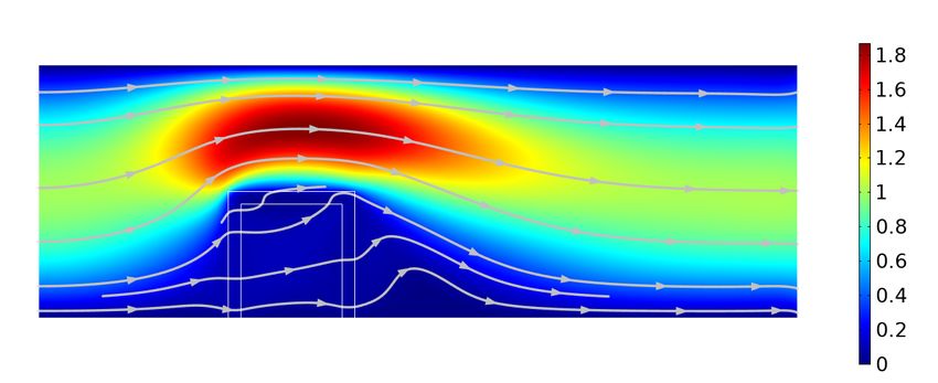
2                                                                                                    Joe Alexandersen

have been made available, often together with educa-         herein are rather sparse on purpose and the reader is re-
tional articles explaining their use. The first published    ferred to the recent review paper instead (Alexandersen
code was the famous “99-line” MATLAB code by Sig-            and Andreasen, 2020).
mund (2001), used broadly around the world in teach-              This article provides a step-by-step introduction to
ing and initial experiments with topology optimisation.      all the needed steps, along with a relatively simple and
Subsequently, this code was updated to a more effi-          efficient implementation in MATLAB - where compati-
cent “88-line” version by Andreassen et al. (2011) and       bility of the main files with the open-source alternative
most recently a hyper-efficient “neo99” version by Fer-      GNU Octave has been ensured. The code presented in
rari and Sigmund (2020). Over the years, many edu-           this paper builds on the “88-line” code by Andreassen
cational codes have been published for topology op-          et al. (2011) and uses the same basic code structure and
timisation using e.g. level set methods (Challis, 2010;      variable names.
Wei et al., 2018), unstructured polygonal meshes (Tal-
ischi et al., 2012), energy-based homogenisation (Xia
and Breitkopf, 2015), truss ground structures (Zegard        1.3 Paper layout
and Paulino, 2014) and large-scale parallel computing
(Aage et al., 2015). The recent review paper by Wang         The article is structured as follows:
et al. (2021) provides a comprehensive overview of edu-       – Section 2 introduces the design representation used
cational articles in the field of structural and multidis-      for density-based topology optimisation of fluid flow
ciplinary optimisation.                                         problems;
                                                              – Section 3 presents the physical formulation and an
                                                                in-depth investigation of the error convergence for
1.2 Fluid flow                                                  important problem parameters;
                                                              – Section 4 details the finite element discretisation
The density-based topology optimisation approach was            and the state solution procedure used;
extended to the design of Stokes flow problems by Bor-        – Section 5 discusses the optimisation formulation,
rvall and Petersson (2003) and further to Navier-Stokes         sensitivity analysis and design solution procedure;
flow by Gersborg-Hansen et al. (2005). Since those sem-       – Section 6 introduces the two benchmark examples
inal papers, topology optimisation has been applied to a        included in the code;
large range of flow-based problems. The recent review         – Section 7 presents a description of the accompany-
paper by Alexandersen and Andreasen (2020) details              ing MATLAB implementation;
the many contributions to this still rapidly developing       – Section 8 shows results obtained using the code for
field. Topology optimisation of pure fluid flow has now         the benchmark examples;
become reasonably mature, with only minor recent con-         – Section 9 discusses modifications to the code for
tributions for steady laminar flow (Alexandersen and            solving more advanced problems;
Andreasen, 2020). Therefore, research efforts should be       – Section 10 discusses the computational time and
focused on building further upon this technology, call-         memory usage;
ing for an educational article and a simple code that         – Section 11 presents concluding remarks.
allows for quickly getting started and skipping initial
repetitive implementations.
                                                             2 Design representation
    Pereira et al. (2016) presented an extension of their
polygonal mesh code (Talischi et al., 2012) to Stokes        This section describes the design representation intro-
flow topology optimisation. Whereas Pereira et al. (2016)    duced to model solid domains immersed in a fluid, al-
focused on stable discretisations of polygonal elements      lowing for density-based topology optimisation. First,
for Stokes flow, this educational article focuses on giv-    the true separated discrete domains that should be rep-
ing a detailed and complete introduction to density-         resented are introduced, and secondly, a continuous de-
based topology optimisation of fluid flow problems gov-      sign representation is described.
erned by the Navier-Stokes equations. The aim is to
serve as the first point of contact for new students and
researchers to quickly get started in the research area      2.1 Discrete separate domains
and to skip many of the initial steps, often consum-
ing unnecessarily long time from the scientific advance-     Figure 1a shows an arbitrary example of a truly discrete
ment of the field. The goal is not to give an overarching    problem with separated fluid and solid domains, de-
overview of the literature on the subject, so references     noted as Ωf and Ωs , respectively. Both Ωf and Ωs can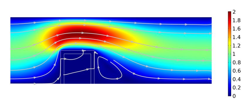
A detailed introduction to density-based topology optimisation of fluid flow problems                                     3

                                                                transition region of intermediate design field values as
                                                                shown in Figure 1b. Generally, during the optimisation
                                                                process there will be many regions of intermediate val-
                                                                ues, whereas a converged design will have significantly
                                                                less, if any – depending on various details as will be
                                                                discussed later. By coupling the continuous design rep-
                                                                resentation to coefficients of the governing equations,
                                                                it is possible to model an immersed geometry which is
                                                                implicitly defined by the design field.

                                                                3 Physical formulation
            (a) Discrete separation of domains
                                                                This section presents the physical formulation of the
                                                                fluid flow problems treated in this article. The Navier-
                                                                Stokes equations are the governing equations and a so-
                                                                called Brinkman penalty term is introduced to facilitate
                                                                density-based topology optimisation.

                                                                3.1 Governing equations

                                                                This article restricts itself to steady-state laminar and
                                                                incompressible flow, governed by the Navier-Stokes equa-
                                                                tions:
           (b) Continuous design representation

                                                                    ∂ui       ∂     ∂ui     ∂uj       ∂p
                                                                ρuj     −µ               +         +     − fi = 0     (2a)
                                                                    ∂xj      ∂xj ∂xj        ∂xi      ∂xi
Fig. 1: Arbitrary computational domain consisting of
fluid and solid domains.                                                                                  ∂ui
                                                                                                               =0    (2b)
                                                                                                          ∂xi
                                                                where ui is the i-th component of the velocity vector
be comprised as the union of non-overlapping subdo-
                                                                u, p is the pressure, ρ is the density, µ is the dynamic
mains, as illustrated for Ωs in Figure 1a. The interface
                                                                viscosity, and fi is the i-th component of the body force
between the solid and fluid domains is clearly defined
                                                                vector f. The Reynolds number is commonly used to
due to the separation of the two domains.
                                                                describe a flow and is defined as:
                                                                       ρU L
                                                                Re =                                                    (3)
2.2 Continuous relaxed representation                                   µ
                                                                where U and L are the reference velocity and length-
In order to perform density-based topology optimisa-
                                                                scale, respectively. The Reynolds number describes the
tion using gradient-based methods, the discrete repre-
                                                                ratio of inertial to viscous forces in the fluid: if Re < 1,
sentation must be relaxed. Firstly, a spatially-varying
                                                                the flow is dominated by viscous diffusion; if Re > 1,
field, γ(x), is introduced, which will be termed the de-
                                                                the flow is dominated by inertia.
sign field. It is equivalent to the characteristic function
of the fluid domain Ωf :
                                                               3.2 Brinkman penalty term
           1 if x ∈ Ωf
γ(x) =                                                  (1)
           0 if x ∈ Ωs                                          In order to facilitate topology optimisation, an artificial
Secondly, the design field is relaxed from binary val-          body force is introduced, termed the Brinkman penalty
ues to a continuous field, allowing intermediate values:        term:
γ(x) ∈ [0; 1]. Figure 1b shows a continuous relaxed rep-        fi = −αui                                               (4)
resentation of the discrete separated domains of Figure
1a. The continuous representation has an implicit rep-          which represents a resistance term and a momentum
resentation of the solid-fluid interface, represented by a      sink, drawing energy from the flow. The Brinkman penalty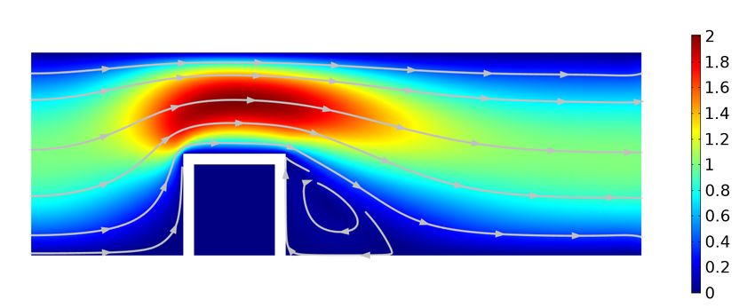
4 Joe Alexandersen
factor, α, is a spatially-varying parameter defined as
follows for the separated domains introduced in Figure
1a:
0 if x ∈ Ωf
α(x) = (5)
∞ if x ∈ Ωs
where the 0 in the fluid domain recovers the original
equations and the infinite value inside the solid domain
theoretically ensures identically zero velocities. This al-
lows for extending the Navier-Stokes equations to the
entire computational domain:
∂ui ∂ ∂ui ∂uj
ρuj −µ +
∂xj ∂xj ∂xj ∂xi
∂p
+ + α (γ(x)) ui = 0
∂xi for x ∈ Ω
∂ui ∂uj ∂ui
+ = 0 Fig. 2: Interpolation of α for various qα .
∂xj ∂xi ∂xi
(6)
physical reflections are required. However, as it will be
where solid domains are modelled as immersed geome- discussed in Sections 3.2.2 and 3.2.3 and shown in Sec-
tries through the Brinkman penalty term. tion 3.3, it is highly relevant to couple the parameters
The Brinkman penalty term can be interpreted in to the physical interpretations to ensure correct scaling
three different ways: of the equations.
1. Volumetric penalty term to ensure zero velocities in
the solid regions 3.2.1 Numerical relaxation
2. Friction term from out-of-plane viscous resistance
3. Friction term from an idealised porous media In practise, the bounds of the Brinkman penalty fac-
tor are defined as follows, based on the design field, γ,
The first interpretation is a purely algorithmic approach, introduced in Figure 1b:
where the only purpose is to simulate an immersed fully
solid geometry inside a fluid domain. The second and αmin if γ(x) = 1
α(γ(x)) = (7)
third are both physical interpretations, but require dif- αmax if γ(x) = 0
ferent lower and upper bounds of Equation 5 formulated For numerical reasons, a finite value must be used in
based on physical parameters. The second interpreta- the solid domain, αmax , being large enough to ensure
tion is limited to only two-dimensional problems, where negligible velocities but small enough to ensure sta-
the computational domain has a finite and relatively bility. The choice of this maximum value will be dis-
small out-of-plane thickness. The first and third inter- cussed in Sections 3.2.3 and 3.3. Furthermore, if two-
pretations can be applied to three-dimensional prob- dimensional problems with a finite out-of-plane thick-
lems. ness are treated, a minimum value, αmin , should remain
The seminal work by Borrvall and Petersson (2003) to account for the out-of-plane viscous resistance as dis-
for Stokes flow and Gersborg-Hansen et al. (2005) for cussed in Section 3.2.2.
Navier-Stokes flow, both introduced a design parametri- In order to interpolate between solid and fluid do-
sation based on the out-of-plane channel height for two- mains, the Brinkman penalty factor is interpolated us-
dimensional problems following the second interpreta- ing the following function:
tion above. Both works also note the comparison to the
1−γ
third interpretation and Gersborg-Hansen et al. (2005) α(γ) = αmin + (αmax − αmin ) (8)
argues for the first interpretation as the ultimate goal of 1 + qα γ
topology optimisation for fluid flow. The recent review where qα is a parameter determining the shape of the
paper by Alexandersen and Andreasen (2020) shows interpolation, as illustrated in Figure 2 for αmin = 0 and
that the dominant interpretation is the first, a purely αmax = 104 . This function is not the same as introduced
algorithmic approach to ensure zero velocities. This is by Borrvall and Petersson (2003), but rather the Ra-
because it easily extends to three-dimensions and no tional Approximation of Material Properties (RAMP)A detailed introduction to density-based topology optimisation of fluid flow problems 5
function (Stolpe and Svanberg, 2001). This ensures a 3.2.4 Note on physical interpretations
linear interpolation is directly achieved by setting qα to
0, whereas the function used by Borrvall and Petersson It is easily seen from Equations 9 and 10, that the two
(2003) only has the linear case as an asymptotic limit. physical interpretations are analogous by connecting
Effectively, qα herein is the inverse of the q used by the permeability to the out-of-plane thickness:
Borrvall and Petersson (2003).
2h2
κ= (11)
5
3.2.2 Minimum penalty factor
as noted by both Borrvall and Petersson (2003) and
The seminal work by Borrvall and Petersson (2003) Gersborg-Hansen et al. (2005).
for Stokes flow and Gersborg-Hansen et al. (2005) for
Navier-Stokes flow, introduced topology optimisation 3.2.5 Dissipated energy
of fluid flow problems using a design parametrisation
based on the out-of-plane channel height for two-dimensionalThis article focuses on minimising the dissipated energy
problems. By assuming parallel plates distanced 2h apart by a flow through a channel structure. The dissipated
and a fully-developed pressure-driven flow (Poiseuille energy due to viscous resistance is defined as:
flow), an out-of-plane parabolic velocity profile is as- 1
Z
∂ui ∂ui ∂uj
sumed between the two plates. This allows for ana- φ = µ + dV (12)
2 Ωf ∂xj ∂xj ∂xi
lytical through-thickness integration, yielding an addi-
tional term to the momentum equations from the out- The dissipated energy is often used as the objective
of-plane viscous resistance in the form of Equation 4. functional of topology optimisation and it is, thus, rel-
When treating two-dimensional problems with a finite evant to investigate the accuracy of this measure when
out-of-plane thickness and lateral no-slip walls, the min- using the Brinkman penalty method.
imum Brinkman penalty must be set to:
5µ
αmin = (9) 3.3 Effect of varying parameters
2h2
where h is half of the domain thickness. However, when This section presents the effect of varying the Reynolds
treating three-dimensional problems, the minimum Brinkman number Re and Brinkman penalty factor α on the ac-
penalty factor should be set to 0 to recover the original curacy of the Brinkman-penalised Navier-Stokes equa-
unencumbered Navier-Stokes momentum equations. tions.
3.2.3 Maximum penalty factor 3.3.1 Example setup
Finding the correct maximum penalty factor is not triv- Figure 3 presents the problem setup used to explore
ial. It must be large enough to ensure negligible flow the accuracy of the Brinkman-penalised Navier-Stokes
through solid regions, but small enough to ensure nu- equations. A hollow box obstacle is placed inside a chan-
merical stability. While the Brinkman term is often seen nel, where a fully-developed parabolic flow with a max-
purely as a volumetric penalty approach for imposing imum of Uin enters at the left-hand side inlet and exits
the no-flow conditions inside the solid, it is beneficial at the right-hand side zero normal-stress outlet. This
to ensure consistent dimensional scaling of the penalty model will be solved using both a discrete design rep-
factor. This can be done by relating it to the friction resentation, modelling only the fluid domain, and a
factor from a fictitious porous media: continuous design representation, with the Brinkman-
µ penalised Navier-Stokes equations in the entire compu-
αmax = (10)
κ tational domain. The same locally-refined mesh is used
where κ is the permeability of the fictitious porous me- for both models to ensure that the discretisation error
dia. This permeability must then be small enough to does not affect the comparison in a significant sense.
ensure negligible velocities inside the solid regions, but The porous media definition in Equation 10 is cho-
as will be shown in Section 8.1.3, the minimum dis- sen for the Brinkman penalty factor and the problem
sipated energy optimisation is pretty forgiving. For a is non-dimensionalised by setting the inlet velocity to
given constant permeability, Equation 10 ensures an al- Uin = 1, the density to ρ = 1, the dynamic viscosity to
most constant ratio between the order of magnitude for µ = 1/Re, and the permeability to κ = Da. The Darcy
the velocities in the flow and solid regions for a range number, Da = Lκ2 , is the non-dimensional permeability.
of Reynolds numbers, as demonstrated in Section 3.3. The Reynolds and Darcy numbers will be varied.6 Joe Alexandersen
For fluid dissipation problems, this is not really an issue
because this pressure is not important for the overall
dissipation and since disconnected fluid regions never
occur in the optimised designs. But for fluid-structure-
interaction, where the fluid exerts a pressure on the
solid, the internal non-zero pressure can be an issue
(Lundgaard et al., 2018).
3.3.3 Error convergence study
(a) Domain and boundary definitions
To clearly show the convergence of the approximate so-
lution from the continuous representation towards the
true solution from the discrete representation, a number
of error measures are computed. The spatial average of
the velocity magnitude inside the solid structure and
inside the cavity are computed as:
Z
1
εu,s = kuk2 dV (13a)
|Ωs | Ωs
(b) Dimensionless lengths Z
1
εu,c = kuk2 dV (13b)
Fig. 3: Problem setup for the example used in Section |Ωc | Ωc
3.3. These are seen as directly equivalent to a relative error
measure, since the true solution for these quantities are
zero and the reference (inlet) value is 1. Furthermore,
3.3.2 Fluid solution the relative error is found for the dissipated energy and
the pressure drop:
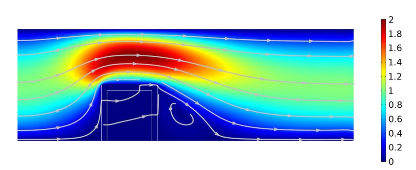
Figure 4 shows the velocity magnitude and pressure
fields using the discrete design representation for Re = |φdisc − φcont |
εφ = (14a)
20. Since the fluid cavity inside the solid structure is dis- φdisc
connected, the pressure is here set equal to a reference
|∆pdisc − ∆pcont |
pressure of 0. It can be seen that the flow moves above ε∆p = (14b)
the obstacle and leaves a re-circulation zone behind it. ∆pdisc
Figure 5 shows the velocity magnitude field using where subscripts ‘disc’ and ‘cont’ denote discrete and
the Brinkman approach for Re = 20 and Da ∈ {10−4 , continuous design representations, respectively, φ is the
10−6 , 10−8 }. For the highest permeability case, Da = dissipated energy of the fluid subdomain defined in Equa-
10−4 , it is seen that a significant amount of fluid passes tion 12 and ∆p is the pressure drop from inlet to outlet
through the solid structure and clearly non-zero veloci- as computed from:
ties exist in the cavity. When this is increased to Da = 1
Z
1
Z
10−6 , the flow solution becomes more accurate, but the ∆p = p dS − p dS (15)
|Γin | Γin |Γout | Γout
recirculation zone behind the obstacle is not fully cap-
tured. This is improved for the last case, Da = 10−8 , Figure 7 shows the error measures as a function of
but even here flow is passing through the obstacle. This the Darcy number for Re = 20. It is clearly seen that
will always be the case for the Brinkman penalty ap- the velocity error measures converge at an order of 1
proach, but the velocities can be driven towards zero and the pressure and dissipation measures at an order
by decreasing the permeability sufficiently. of 1⁄2. This shows that compared to the velocity field,
Figure 6 shows the pressure field using the Brinkman the pressure field needs a significantly higher Brinkman
approach for Re = 20 and Da ∈ {10−4 , 10−6 , 10−8 }. penalty factor to reach a certain accuracy. The dissi-
Due to the continuous nature of the design representa- pated energy also requires a larger Brinkman penalty
tion, pressure gradients exist inside the solid structure factor to achieve a certain accuracy. However, this is
and a non-zero pressure exists in the cavity. The cavity not necessarily important for minimum dissipated en-
pressure approximately becomes the mean of the high ergy optimisation as will be demonstrated in Section
and low surface pressures - for this case ≈ (4+0)/2 = 2. 8.1.3. Additional accuracy becomes important if theseA detailed introduction to density-based topology optimisation of fluid flow problems 7
(a) Velocity magnitude (b) Pressure field
Fig. 4: Velocity magnitude and pressure fields using the discrete design representation for Re = 20.
(a) Da = 10−4 (a) Da = 10−4
(b) Da = 10−6 (b) Da = 10−6
(c) Da = 10−8 (c) Da = 10−8
Fig. 5: Velocity magnitude fields using the Brinkman Fig. 6: Pressure fields using the Brinkman approach for
approach for Re = 20 and Da ∈ {10−4 , 10−6 , 10−8 }. Re = 20 and Da ∈ {10−4 , 10−6 , 10−8 }.
functionals are used as constraints where the limit rep- of the pressure field is also very important if it is used
resents a physical value. The constraint looses its physi- to drive additional physics, such as fluid-structure in-
cality, if the functional is not resolved to a large enough teraction (FSI) which was clearly shown by Lundgaard
accuracy1 . However, if treated in relative terms as in et al. (2018).
Section 9.2.2, then this is less of an issue. The accuracy Figure 8 shows the error measures as a function
1
of the Reynolds number for Da = 10−6 . It can be
This is very similar to stress constraints in structural
seen that defining the Brinkman penalty factor using
topology optimisation, where a maximum stress limit be-
comes meaningless, unless the stresses and aggregated maxi- Equation 10 ensures a constant error for a range of
mum is accurate Le et al. (2010); da Silva et al. (2019). Reynolds numbers. However, as the Reynolds number8 Joe Alexandersen
Fig. 9: Element degrees-of-freedom (DOFs) and nodal
numbering.
moderate Reynolds numbers treatable with the present
steady-state implementation. An alternative scaling law
proposed by Kondoh et al. (2012) is discussed in Ap-
pendix A.
4 Discretisation and solution
Fig. 7: Error measures as a function of permeabil-
ity for a Reynolds number of Re = 20 and Da ∈ 4.1 Finite element formulation
{10−2 , 10−3 , 10−4 , 10−5 , 10−6 , 10−7 , 10−8 } .
The governing equations in Equation 2 are discretised
using a stabilised continuous Galerkin finite element
formulation. Both the velocity and pressure fields are
approximated using piecewise bi-linear interpolation func-
tions and the design field is approximated using piece-
wise constant values, rendering a u1p1g0 element as
shown in Figure 9. This yields 8 velocity degrees-of-
freedom (DOFs), 4 pressure DOFs, and 1 design DOF
per element. Due to the equal-order interpolation for ve-
locity and pressure, Pressure-Stabilising Petrov-Galerkin
(PSPG) stabilisation is applied to get a stable finite ele-
ment formulation. Furthermore, to avoid spurious oscil-
lations due to convection, Streamline Upwind Petrov-
Galerkin (SUPG) stabilisation is also applied. The de-
tailed formulation is given in Appendix B.
The discretisation gives rise to a non-linear system
of equations, which is posed in residual form:
r(s, γ) = A(s, γ) s = 0 (16)
T T T
Fig. 8: Error measures as a function of Reynolds num- where A is the system coefficient matrix, s = u p
ber for a Darcy number of Da = 10−6 and Re ∈ is the vector of global state DOFs, u is the vector of
{0.01, 0.1, 1, 5, 10, 50, 100, 150}. velocity DOFs, p is the vector of pressure DOFs, and
γ is the vector of design field values. There are many
non-linear and design-dependent terms in the system:
becomes larger than 10, the error begins to slowly grow. the convection term is dependent on the velocity field;
This makes sense, since the porous media analogy is the Brinkman term is dependent on the design field; and
based on scaling with the viscous diffusion term and a the stabilisation terms are dependent on both the veloc-
Brinkman porous media model. As the Reynolds num- ity and design field (either directly through convection
ber increases, the convective term begins to dominate in and Brinkman terms or indirectly through the stabili-
Equation 6 and, thus, it makes sense that the penalty sation parameter). Thus, a robust non-linear solver is
term should scale differently. However, the slight in- needed and the Newton solver is detailed in the subse-
crease in the errors are not seen as significant for the quent section. Furthermore, derivation of accurate par-A detailed introduction to density-based topology optimisation of fluid flow problems 9
tial derivatives, such as the Jacobian matrix and those 5 Optimisation formulation
necessary for optimisation, can be cumbersome. There-
fore, these derivatives will be automatically computed 5.1 Objective functional
using the Symbolic Toolbox in MATLAB.
The dissipated energy was originally introduced as the
objective functional by Borrvall and Petersson (2003).
Equation 12 is the dissipated energy in the fluid do-
4.2 Newton solver main due to viscous resistance only. The addition of the
Brinkman penalty term introduces a body force, which
To solve the non-linear system of equations, a damped must be taken into account in the dissipated energy:
Newton method is used. At each non-linear iteration, k,
the following linearised problem is solved for the New- 1
Z
∂ui ∂ui ∂uj
ton step, ∆sk : φ= µ + + α(x)ui ui dV (20)
2 Ω ∂xj ∂xj ∂xi
∂r
∆sk = −r(sk−1 ) (17) which is now integrated over the entire computational
∂s k−1 domain.
where the solution is then updated according to:
5.2 Volume constraint
sk = sk−1 + δk ∆sk (18)
In order to avoid trivial solutions, a maximum allowable
with δk ∈ [0.01; 1] being the damping factor2 . In or- volume of fluid is imposed as a constraint. The relative
der to gain robust convergence for moderate Reynolds volume of fluid is in continuous form defined as:
numbers, the damping factor is updated according to
the minimum of a quadratic fit of the residual norm
Z
1
V = γ(x) dV (21)
dependence on δ. The residual and its 2-norm is calcu- |Ω| Ω
lated for δ ∈ {0, 0.5, 1}, with the current value (δ = 0)
already known. A quadratic equation is then fitted to which represents the volumetric average of the design
the residual norms with the unique minimising damp- field. The relative fluid volume should be restricted to
ing factor expressed analytically. The damping factor is be below Vf ∈]0; 1[, which is the fraction of the total
then set to: domain allowed to be fluid. After discretisation as de-
scribed in Section 4, the relative volume is computed
3||r0 ||2 − 4||r0.5 ||2 + ||r1 ||2 by:
δk = max 0.01, min 1,
4||r0 ||2 − 8||r0.5 ||2 + 4||r1 ||2
nel
(19) 1 X
V = γe (22)
nel e=1
where rδ is the residual evaluated for the solution up-
dated with a given δ. where nel is the number of elements and it has been
The Newton solver is run until the current resid- exploited that all elements have the same volume in
ual norm has been reduced relative to the initial be- the current implementation.
low a predefined threshold. To speed up convergence,
the state solution from the previous design iteration is
used as the initial solution for the Newton solver. If the
solver does not converge before a maximum iteration 5.3 Optimisation problem
number is reached, it tries again from a zero (except
for boundary conditions) initial solution. If that also The final discretised optimisation problem is:
fails, the Reynolds number may be too large to have a
steady-state solution for the problem. It is also possible minimise: fφ (s(γ), γ) = φ
γ
that the problem is so non-linear, that it might need
subject to: V (γ) ≤ Vf (23)
ramping of the inlet velocity or Reynolds number.
with: r(s(γ), γ) = 0
2
The lower bound is chosen to avoid stagnation. 0 ≤ γi ≤ 1, i = 1, . . . , nel10 Joe Alexandersen
5.4 Adjoint sensitivity analysis by the negative gradients (more fluid is better). How-
ever, this has worked extremely well for the problems
The gradients of any functionals dependent on the state at hand, because mostly the dissipated energy gradients
field are found using adjoint sensitivity analysis. A gen- are negative.
eral description is given in Appendix C. The sensitivi- The Lagrange multiplier is found using bisection. To
ties for a generic functional f are found from: speed up the process, the upper bound estimate sug-
df ∂f ∂r gested by Ferrari and Sigmund (2020) is modified for
= − λT (24) η = 13 :
dγe ∂γe ∂γe
where λ is the vector of adjoint variables for the state
ne ∂φ
! 31 3
¯l = 1 ∂γe
X
residual constraint found from the adjoint problem: γe − ∂V
(29)
nel Vf e=1 ∂γe
∂r T ∂f T
λ= (25)
∂s ∂s
5.6 Continuation scheme
The above is valid for any equation system formulated
as a residual, r, and any state-dependent functional, f ,
As shown by Borrvall and Petersson (2003), the min-
be it objectives or constraints. For a given system, two
imisation of dissipated energy is self-penalising for the
partial derivatives of the residual are necessary, and for
Brinkman approach with linear interpolation of α(γ).
a given functional, two partial derivatives of the func-
This means that intermediate design values are not ben-
tional are necessary: with respect to the design field and
eficial and the optimal solutions are discrete 0-1. How-
the state field. These partial derivatives can be found
ever, it is often beneficial to relax the problem using
analytically by hand, but in the presented implementa-
the interpolation factor, qα , in the initial stages of the
tion they are found automatically using symbolic dif-
optimisation process in order to avoid convergence to
ferentiation in MATLAB.
particularly poor local minima. Therefore, it is common
to solve the minimisation problem for a sequence of qα ,
5.5 Optimality criteria optimiser known as a continuation scheme.
In the presented code, a heuristic approach is imple-
An optimality criteria (OC) based optimisation algo- mented to automatically choose the interpolation fac-
rithm is used in the presented code. The implemented tor. The sequence for the continuation scheme is given
OC method is the modified version suggested by Bendsøe by:
and Sigmund (2004) for compliant mechanism prob-
q0 q0 q0
lems, where the design gradients can be both positive qα ∈ qα0 , α , α , α (30)
2 10 20
and negative:
where:
if γe Be η ≤ γeL
L
γe
new
γe = γe U
if γe Be η ≥ γeU (26) (αmax − α0 ) − x0 (αmax − αmin )
qα0 = (31)
η
γe Be otherwise x0 (α0 − αmin )
is the initial interpolation factor necessary to ensure an
where η = 13 is a damping factor and the upper bounds
initial Brinkman penalty of α0 for an initial design field
at each iteration are given as:
value of x0 . The interpolation factor is changed when
γeL = max(0, γe − m) (27a) the subproblem is considered converged or after a pre-
defined number of design iterations. For the problems
γeU = min(1, γe + m) (27b) implemented in the presented code, an initial Brinkman
with m being the movelimit. The optimality criteria penalty of α0 = 2.5µ
0.12 works very well. However, do bear
ratio is given as: in mind that this is a heuristic value and will not work
for all problems and all settings.
∂φ
!
− ∂γ e
Due to the non-convexity, the initial Brinkman penalty
Be = max ε, ∂V (28) of the domain plays an important role in which direc-
l ∂γe
tion the design will progress. The initial flow field de-
where ε is a small positive number (e.g. 10−10 ) and l termines the exploration of the design space, because if
is the Lagrange multiplier for the volume constraint. the flow is not moving through some parts of the design
This means that positive gradients (less fluid is bet- domain, sensitivities will often be near zero in those ar-
ter) are ignored and the design process is driven only eas. Therefore, it is often beneficial to start with anA detailed introduction to density-based topology optimisation of fluid flow problems 11
Fig. 10: Problem setup for the double pipe problem.
initial Brinkman penalty that allows for the fluid to Fig. 11: Problem setup for the pipe bend problem.
move into most areas of the domain. This was for in-
stance recently observed in the topology optimisation
of heat exchanger designs by Høghøj et al. (2020).
6 Benchmark examples
(a) Local nodal numbering
6.1 Double pipe problem
This problem was first introduced by Borrvall and Pe-
tersson (2003) and is illustrated in Figure 10. On the
left-hand side, there are two inlets at which parabolic
normal velocity profiles are prescribed with a maximum
velocity of Uin . On the right-hand side, there are two
zero-pressure outlets at which the flow is specified to
(b) Global nodal and element numbering
exit in the normal direction. This is a more realistic
boundary condition traditionally used in the compu- Fig. 12: Local and global numbering. Numbers with-
tational fluid dynamics community, compared to pre- out circles indicate nodal numbering and number with
scribed parabolic flow profiles at the outlets (Borrvall circles indicate element numbering.
and Petersson, 2003). However, this does introduce new
and better minima as was shown by Papadopoulos et al.
(2021), which makes the problem more difficult. 7 MATLAB implementation
7.1 Mesh and numbering
6.2 Pipe bend problem
Figure 12 shows the local and global numbering used
This problem was also introduced by Borrvall and Pe- in the presented implementation. As shown in Figure
tersson (2003) and is illustrated in Figure 11. On the 12b, for the global numbering of both the nodes and el-
left-hand side, there is an inlet at which a parabolic ements begins in the upper-left corner, increasing from
normal velocity profile is prescribed with a maximum top to bottom and then from left to right. The origin of
velocity of Uin . On the bottom, there is a zero-pressure the global coordinate system is placed in the upper-left
outlet at which the flow is specified to exit in the normal corner, with the first spatial direction, x1 , being posi-
direction - a minor change from Borrvall and Petersson tive from left to right and the second spatial direction,
(2003) as for the double pipe problem. x2 , being positive from top to bottom. This orientation12 Joe Alexandersen
has been chosen to simplify easy plotting of the various % PHYSICAL PARAMETERS 15
spatial fields in MATLAB. The velocity and pressure Uin = 1e0; rho = 1e0; mu = 1e0; 16
DOFs follow the ordering of the nodes and the design
field follows the ordering of the elements. The maximum and minimum Brinkman penalty fac-
tors are per default defined with respect to an out-of-
plane thickness according to Equation 9 (Borrvall and
7.2 Brief description of code Petersson, 2003) and the heuristic continuation scheme
is automatically computed and stored in qavec:
The full code consists of multiple files, the main ones of % BRINKMAN PENALISATION 17
which are available in Appendices D-H. The full code alphamax = 2.5*mu/(0.01ˆ2); alphamin = ... 18
base is available on GitHub (Alexandersen, 2022). 2.5*mu/(100ˆ2);
The main file topFlow.m (Appendix D) can be di- % CONTINUATION STRATEGY 19
ainit = 2.5*mu/(0.1ˆ2); 20
vided into three parts: pre-processing, optimisation loop, qinit = (−xinit*(alphamax−alphamin) − ... 21
and post-processing. Each part will be very briefly de- ainit + ...
scribed herein, except the definition of problem param- alphamax)/(xinit*(ainit−alphamin));
eters which is treated in detail below since this will be qavec = qinit./[1 2 10 20]; qanum = ... 22
length(qavec); conit = 50;
of importance to the subsequent definition of examples
and results. A detailed description of the code is avail- where ainit is the initial Brinkman penalty, qinit is
able in the Supplementary Material. the initial interpolation factor computed using Equa-
tion 31, qanum is the number of continuation steps, and
7.2.1 Definition of input parameter (lines 6-29) conit is the maximum number of iterations per contin-
uation step.
The pre-processing part starts with the setting of in-
Various optimisation parameters are then defined:
put parameters (lines 6-29) to define the problem and
optimisation parameters. In the presented code, two % OPTIMISATION PARAMETERS 23
maxiter = qanum*conit; mvlim = 0.2; ... 24
different problems are already implemented and the plotdes = 0;
probtype variable determines which one is to be op- chlim = 1e−3; chnum = 5; 25
timised:
7 % PROBLEM TO SOLVE (1 = DOUBLE PIPE; 2 = ... where maxiter is the maximum number of total design
PIPE BEND) iterations, mvlim is the movelimit m for the OC update,
8 probtype = 1; chlim is the stopping criteria, chnum is the number of
Next the dimensions of the domain and the discretisa- subsequent iterations the convergence criteria must be
tion are given: met, and plotdes is a Boolean determining whether to
plot the design during the optimisation process (0 =
9 % DOMAIN SIZE no, 1 = yes).
10 Lx = 1.0; Ly = 1.0;
11 % DOMAIN DISCRETISATION The parameters for the Newton solver are defined:
12 nely = 30; nelx = nely*Lx/Ly;
% NEWTON SOLVER PARAMETERS 26
where Lx and Ly are the dimensions in the x - and y- nltol = 1e−6; nlmax = 25; plotres = 0; 27
directions, respectively. The number of elements in the
x-direction, nelx, is automatically determined from the where nltol is the required residual tolerance for con-
supplied number of elements in the y-direction, nely, to vergence, nlmax is the maximum number of non-linear
ensure square elements. The implementation can handle iterations, and plotres is a Boolean determining whether
rectangular elements, so nelx can be decoupled from to plot the convergence of the residual norm over the
nely if necessary. optimisation process (0 = no, 1 = yes).
The allowable volume fraction Vf is stored in the Finally, the option to export the contour of the final
volfrac variable and the initial design field value is set design as a DXF (Data Exchange Format) file can be
to be the same to fulfill the volume constraint from the activated:
start: % EXPORT FILE 28
filename='output'; exportdxf = 0; 29
13 % ALLOWABLE FLUID VOLUME FRACTION
14 volfrac = 1/3; xinit = volfrac;
where filename is a specified filename and exportdxf
The inlet velocity Uin is stored in the variable Uin and is a Boolean determining whether to export the design
the fluid density, ρ and dynamic viscosity, µ, are stored (0 = no, 1 = yes).
in the variables rho and mu, respectively:A detailed introduction to density-based topology optimisation of fluid flow problems 13
7.2.2 Other pre-processing (lines 30-66) Parameter Value Code
Lx 1 Lx = 1.0
Ly 1 Ly = 1.0
Subsequently, various arrays are defined (lines 30-44) ρ 10−3 rho = 1e-3
for the quick assembly of the matrices and vectors from µ 1 mu = 1.0
αmax 2.5µ/(0.012 )
the finite element analysis based on the sparse function alphamax = 2.5*mu/(0.01^2)
αmin 2.5µ/(1002 ) alphamin = 2.5*mu/(100^2)
in MATLAB. The boundary conditions for the avail- 1/3
Vf volfrac = 1/3
able problems are defined in the separate MATLAB nex 102 nelx = 102
file problems.m (Appendix E) and matrices for quick ney 102 nely = 102
enforcement of Dirichlet conditions are built (lines 45-
51). Finally, various arrays, counters and constants are Table 1: Parameter values used for double pipe solu-
initialised (lines 52-66). tions in Figures 13 and 14.
7.2.3 Optimisation loop (lines 67-167) 4. Pressure field, p
5. Velocity and design field along a cut-line
Prior to the optimisation loop start, some information
is output to the screen and timers are initiated (lines Finally, if requested by setting exportdxf = 1, the con-
67-73). The optimisation starts using a while loop (line tour of the final optimised design is exported to DXF
74) and computation of the greyscale indicator (Sig- format for verification analysis in external software.
mund, 2007) and material interpolation per Equation 8
(lines 76-80). The non-linear solver loop iteratively up-
dates the solution (lines 81-112) using Newton’s method 8 Examples
according to Section 4.2. The finite element analysis is
carried out according to Section 4.1 (lines 85-93) using 8.1 Double pipe problem
function RES and JAC to build to residual vector and Ja-
This problem was introduced in Section 6.1 and is the
cobian matrix, respectively. For the converged solution,
default for the provided code when probtype = 1. It
the objective functional is evaluated (line 114) using the
was originally introduced by Borrvall and Petersson
function PHI according to Section 5.1 and the volume
(2003) for Stokes flow, but will herein also be optimised
is evaluated for the current design (line 117) according
for Navier-Stokes flow.
to Section 5.2. The current solution is evaluated (lines
124-126) and if it is not considered converged, then the
adjoint problem is formed and solved (lines 131-136) 8.1.1 Stokes flow
and the sensitivities are computed (lines 137-144) ac-
In order to make the results directly comparable to
cording to Section 5.4. Subsequently, the design field is
those of Borrvall and Petersson (2003), the parameter
updated using the optimality criteria optimiser (lines
values are set as in Table 1. To simulate Stokes flow ide-
145-154) according to Section 5.5. Before repeating the
ally the density would be set to 0, but due to the current
process for the new design, the interpolation parameter
implementation not being able to handle that, the den-
is updated if necessary according to the continuation
sity is set to a small number, ρ = 10−3 instead. This
scheme (lines 155-159) in Section 5.6.
yields an inlet Reynolds number of Rein = 1.67 × 10⁻⁴ ,
The functions for evaluating the residual vector, Ja-
which is sufficiently small to ensure Stokes flow.
cobian matrix, objective functional, and their partial
Figure 13 shows the optimised design and corre-
derivatives, are all automatically built using the file
sponding physical fields for a square domain with Rein =
analyticalElement.m. This script uses the MATLAB
1. From Figure 13b it can be seen that the converged
Symbolic Toolbox to symbolically derive and differen-
design in Figure 13a ensures the lowest and highest
tiate the required vectors and matrices.
Brinkman penalty factor in the fluid region and solid
region, respectively. This results in negligible velocities
7.2.4 Post-processing (lines 168-170) in the solid region with the flow passing easily through
the channels, as seen in Figure 13c. Figure 13d shows
The results are post-processed and plotted in an exter-
the pressure field, where it can be seen that a con-
nal file postproc.m (line 169), where 5 standard plots
tinuous pressure field exists even in the solid region.
are made:
The final objective value is φ = 22.0956, which is very
1. Design field γ(x) close to the value of 25.67 reported by Borrvall and
2. Brinkman penalty field, α(γ(x)) Petersson (2003). Differences can be attributed to dif-
√
3. Velocity magnitude field, U = ui ui ferent implementations, most likely the fact that the14 Joe Alexandersen
Parameter Value Code
ρ 1 rho = 1.0
µ 1/6Re mu = 1/(6*20)
in
Table 2: Updated values used for double pipe solutions
in Figure 15. Other values are given in Table 1.
present uses stabilised linear finite elements in contrast
to mixed-order quadratic-linear elements (Borrvall and
Petersson, 2003). The level of intermediate design vari-
ables since the final interpolation factors are almost the
(a) Design field same, at 9.85 for the present code and an equivalent of
10 in Borrvall and Petersson (2003), and the level of
greyscale is therefore similar.
An elongated domain is investigated by setting Lx =
1.5 similar to Borrvall and Petersson (2003), with the
number of elements increased proportionally in the same
direction. Figure 14 shows the optimised design and cor-
responding physical fields. The optimised design is now
a “double wrench” design, where the channels merge at
the centre to minimise viscous losses along the channel
walls. The final objective value is φ = 23.5732, which
is very close to the value of 27.64 reported by Borrvall
(b) Brinkman penalty field
and Petersson (2003).
8.1.2 Navier-Stokes
In order to non-dimensionalise the problem and con-
trol it using the Reynolds number, Rein , the density is
set to ρ = 1 (rho = 1.0) and the viscosity is set to
µ = 1/6Rein (mu = 1/(6*20)). The 6 in the denomina-
tor ensures that the Reynolds number, Rein , is based
L
on the inlet height which is 6y as shown in Figure 10.
Other parameter values are as previously.
Figure 15 shows the optimised designs obtained for
(c) Velocity magnitude field
increasing Reynolds number. It is observed that for
Rein = 40 and above, the OC solver converges to the lo-
cal minimum of two “straight” channels. It is observed
using COMSOL simulations, that this local minimum
is worse than the double wrench channel for Reynolds
numbers up to 200. The MMA solver introduced in Sec-
tion 9.2.1 is actually able to converge to a significantly
better design for Rein = 40.
8.1.3 Variation of αmax
(d) Pressure field To demonstrate the robustness of the proposed heuris-
tic initial Brinkman penalty and continuation scheme,
Fig. 13: Optimised design and corresponding physical as well as the insensitivity of minimum dissipation opti-
fields for the double pipe problem with Lx = 1 and misation to the maximum Brinkman penalty, the dou-
Rein = 10−3 . Final values: φ = 22.0956 after 63 itera- ble pipe problem will be optimised for Rein = 20 using
tions. 5 additional αmax . Getting to the double wrench chan-
nel for Rein = 20 seems pretty difficult and the poorerA detailed introduction to density-based topology optimisation of fluid flow problems 15
(a) Design field (a) Rein = 20
(b) Brinkman penalty field (b) Rein = 40
Fig. 15: Optimised designs for the double pipe problem
with increasing Reynolds number and Lx = 1.5. Final
values: (a) φ = 0.2126 after 102 iterations; (b) φ =
0.1380 after 59 iterations.
local minima double pipe design is obtained very eas-
ily. Having a constant fixed initial Brinkman penalty,
αinit , of the entire design domain ensures that the same
initial flow field is obtained independent of maximum
(c) Velocity magnitude field
Brinkman penalty, αmax .
The values predicted by the presented MATLAB
code are compared to verification analyses using COM-
SOL of post-processed designs. The export.m file pro-
vides export capabilities of the design field contour to
the DXF file format. The DXF file can then be im-
ported into COMSOL and used to trim the computa-
tional domain. An example COMSOL file is included in
the Supplementary Material.
Figure 16 shows the dissipated energy of the final
optimised designs. The final designs look basically iden-
tical to Figure 15a and are, thus, not shown here. It
(d) Pressure field can be seen that the post-processed performance of
the designs are more or less constant independent of
Fig. 14: Optimised design and corresponding physical αmax . The values predicted by the continuous Brinkman
fields for the double pipe problem with Lx = 1.5 and model are seen to be quite far off for lower maximum
Rein = 10−3 . Final values: φ = 23.5732 after 87 itera- penalties. However, this shows that even a low maxi-
tions. mum Brinkman penalty, which in theory yields a large
error in the prediction of the dissipated energy (Figure16 Joe Alexandersen
Fig. 17: Optimised design for the pipe bend problem
using values from Borrvall and Petersson (2003). Final
values: φ = 9.1862 after 66 iterations.
Fig. 16: Rein = 20
Parameter Value Code
Lx 1 Lx = 1.0
Parameter Value Code Ly 1 Ly = 1.0
Lx 1 Lx = 1.0 ρ 10−3 rho = 1.0
µ 1/(5 Re ) mu = 1/(5*10)
Ly 1 Ly = 1.0 in
ρ 10−3 rho = 1e-3 αmin 2.5µ/(1/52 ) alphamin = 2.5*mu/(1/5^2)
µ 1 mu = 1.0 αmax 104 αmin alphamax = 1e4*alphamin
αmax 2.5µ/(1/0.012 ) alphamax = 2.5*mu/(1/0.01^2) Vf 0.25 volfrac = 0.25
αmin 2.5µ/(1002 ) alphamin = 2.5*mu/(100^2) nex 100 nelx = 100
Vf 0.25 volfrac = 0.25 ney 100 nely = 100
nex 100 nelx = 100
ney 100 nely = 100 Table 4: Parameter values used for pipe bend solution
in Figure 18.
Table 3: Parameter values used for pipe bend solution
in Figure 17.
8.2.1 Stokes flow
7), ends up giving the same or close to the same final In order to make the results comparable to those of
design and performance. This insensitivity was already Borrvall and Petersson (2003), the parameter values are
noted originally by Borrvall and Petersson (2003), but set as in Table 3. As previously, the density is set to a
not explicitly shown. small number, ρ = 10−3 , yielding an inlet Reynolds
number of Rein = 2 × 10⁻⁴ which is small enough to
This conclusion is somewhat disconnected from the approximate Stokes flow.
investigations of the flow accuracy in Section 3.3 and Figure 17 shows the optimised design obtained using
Figure 5. However, in contrast to the reference geome- the values from Borrvall and Petersson (2003) listed in
try in Section 3.3, the final optimised design for mini- Table 3. The design is a straight channel from the inlet
mum dissipated energy do not have re-circulation zones, to the outlet with a final objective value of φ = 22.0956,
since this is detrimental to the energy functional. There- which is very close to the value of 25.67 reported by Bor-
fore, for the optimised designs, a lower maximum Brinkman rvall and Petersson (2003). The streamlines show that
penalty appears to be forgiving. the maximum Brinkman penalty is not large enough to
provide enough resistance to flow through the solid re-
gions. However, as previously shown, while increasing
the αmax may increase the accuracy of the flow mod-
elling, almost identical optimised designs are obtained
8.2 Pipe bend problem for minimum dissipated energy.
This problem was introduced in Section 6.2 and is se- 8.2.2 Navier-Stokes flow
lected in the code by setting probtype = 2. It was orig-
inally introduced by Borrvall and Petersson (2003) for In order to investigate the effect of inertia, the out-of-
Stokes flow and also treated by Gersborg-Hansen et al. plane channel height is set to the width of the inlet. This
(2005) for Navier-Stokes flow. ensures a hydraulic diameter of the inlet width/heightA detailed introduction to density-based topology optimisation of fluid flow problems 17
Fig. 18: Design contours for the pipe bend problem
with increasing Reynolds number. Final values: (a) φ =
2.484 × 10⁻¹ after 58 iterations; (b) φ = 2.830 × 10⁻²
after 63 iterations; (c) φ = 6.502 × 10⁻³ after 40 itera-
tions. Fig. 19: Problem setup for the modified rugby ball prob-
lem.
Optimised for:
Analysed at: Re = 10 Re = 100 Re = 500 9 Modifications
Re = 10 [×10−1 ] 2.484 2.731 3.071
Re = 100 [×10−2 ] 2.889 2.830 3.105
Re = 500 [×10−3 ] 8.459 6.553 6.502 This Section presents a series of extensions to the pro-
vided code, showing how it is possible to extend it to
Table 5: Cross-check table of the optimised designs solve a range of more complicated examples including
for the pipe bend problem shown in Figure 18. Values fixed regions and other objective functionals.
should be multiplied by. The best performing design for
each analysis Reynolds number is highlighted in bold.
9.1 Fixed regions of solid and fluid
and a well-defined Reynolds number. The problem is It is common that the design domain is only a subset of
non-dimensionalised and controlled using the inlet Reynoldsthe computational domain, where the rest is defined as
number, Rein , leading to the parameter values listed in fixed solid or fluid domains. In the discretised problem
Table 4. The 5 in the denominator of the viscosity en- this can be handled by restricting optimisation to the
sures that the Reynolds number is based on the inlet active elements in the defined design domain, with pas-
L
width, which is 5y as shown in Figure 11. sive elements in the fixed domains remaining constant
Figure 18 shows the contours of the optimised de- at their prescribed value.
signs for increasing Reynolds number. For a low Reynolds The implementation of passive and active elements
number, Rein = 10, a more or less straight pipe is will be illustrated using the so-called rugby ball prob-
formed similar to that for Stokes flow. When the Reynolds lem, introduced by Borrvall and Petersson (2003) in the
number increases, inertia begins to play a role and the context of topology optimisation, but it has its roots
curvature of the pipe changes to accommodate this. in the work by Pironneau (1973). Figure 19 shows the
This is confirmed by the cross-check of the three designs external flow problem with a free flow velocity of Uin
with the objective values in Table 5. A cross-check is applied around the entire outer boundary and a single
strictly necessary prior to drawing conclusions from de- zero-pressure point constraint in the upper-left corner.
signs optimised for different conditions. A cross-check A thin region next to the boundary all the way around
is where the optimised designs are tested for the other the outside will be prescribed as fluid regions and a
flow conditions and compared. A successful cross-check solid square will be prescribed in the centre of the do-
is where the design optimised for certain conditions is main. The solid square is not imposed originally, but
also the best for these conditions. This means it has the is done so here to demonstrate the definition of both
lowest value in its own row, such that the diagonal has types of passive domains. Table 6 lists the parameter
the best values as highlighted in bold in Table 5. values used herein.You can also read