ADAPTIVE DISCRETIZATION FOR CONTINUOUS CON- TROL USING PARTICLE FILTERING POLICY NETWORK
←
→
Page content transcription
If your browser does not render page correctly, please read the page content below
Under review as a conference paper at ICLR 2021

A DAPTIVE D ISCRETIZATION FOR C ONTINUOUS C ON -
TROL USING PARTICLE F ILTERING P OLICY N ETWORK

 Anonymous authors
 Paper under double-blind review

                                             A BSTRACT

         Controlling the movements of highly articulated agents and robots has been a
         long-standing challenge to model-free deep reinforcement learning. In this paper,
         we propose a simple, yet general, framework for improving the performance of
         policy gradient algorithms by discretizing the continuous action space. Instead
         of using a fixed set of predetermined atomic actions, we exploit particle filtering
         to adaptively discretize actions during training and track the posterior policy rep-
         resented as a mixture distribution. The resulting policy can replace the original
         continuous policy of any given policy gradient algorithm without changing its un-
         derlying model architecture. We demonstrate the applicability of our approach
         to state-of-the-art on-policy and off-policy baselines in challenging control tasks.
         Baselines using our particle-based policies achieve better final performance and
         speed of convergence as compared to corresponding continuous implementations
         and implementations that rely on fixed discretization schemes.

1   I NTRODUCTION
In the last few years, impressive results have been obtained by deep reinforcement learning (DRL)
both on physical and simulated articulated agents for a wide range of motor tasks that involve learn-
ing controls in high-dimensional continuous action spaces (Lillicrap et al., 2015; Levine et al., 2016;
Heess et al., 2017; Haarnoja et al., 2018c; Rajeswaran et al., 2018; Tan et al., 2018; Peng et al., 2018;
2020). Many methods have been proposed that can improve the performance of DRL for continu-
ous control problems, e.g. distributed training (Mnih et al., 2016; Espeholt et al., 2018), hierarchical
learning (Daniel et al., 2012; Haarnoja et al., 2018a), and maximum entropy regularization (Haarnoja
et al., 2017; Liu et al., 2017; Haarnoja et al., 2018b). Most of such works, though, focus on learning
mechanisms to boost performance beyond the basic distribution that defines the action policy, where
a Gaussian-based policy or that with a squashing function is the most common choice as the basic
policy to deal with continuous action spaces. However, the unimodal form of Gaussian distributions
could experience difficulties when facing a multi-modal reward landscape during optimization and
prematurely commit to suboptimal actions (Daniel et al., 2012; Haarnoja et al., 2017).
To address the unimodality issue of Gaussian policies, people have been exploring more expres-
sive distributions than Gaussians, with a simple solution being to discretize the action space and
use categorical distributions as multi-modal action policies (Andrychowicz et al., 2020; Jaśkowski
et al., 2018; Tang & Agrawal, 2019). However, categorical distributions cannot be directly extended
to many off-policy frameworks as their sampling process is not reparameterizable. Importantly, the
performance of the action space discretization depends a lot on the choice of discrete atomic actions,
which are usually picked uniformly due to lack of prior knowledge. On the surface, increasing the
resolution of the discretized action space can make fine control more possible. However, in prac-
tice, this can be detrimental to the optimization during training, since the policy gradient variance
increases with increasing number of atomic actions (Tang & Agrawal, 2019).
Our work also focuses on action policies defined by an expressive, multimodal distribution. In-
stead of selecting fixed samples from the continuous action space, though, we exploit a particle-
based approach to sample the action space dynamically during training and track the policy rep-
resented as a mixture distribution with state-independent components. We refer to the resulting
policy network as Particle Filtering Policy Network (PFPN). We evaluate PFPN on state-of-the-art
on-policy and off-policy baselines using high-dimensional tasks from the PyBullet Roboschool en-

                                                   1
Under review as a conference paper at ICLR 2021

vironments (Coumans & Bai, 2016–2019) and the more challenging DeepMimic framework (Peng
et al., 2018). Our experiments show that baselines using PFPN exhibit better overall performance
and/or speed of convergence and lead to more robust agent control. as compared to uniform dis-
cretization and to corresponding implementations with Gaussian policies.
Main Contributions. Overall, we make the following contributions. We propose PFPN as a general
framework for providing expressive action policies dealing with continuous action spaces. PFPN
uses state-independent particles to represent atomic actions and optimizes their placement to meet
the fine control demand of continuous control problems. We introduce a reparameterization trick
that allows PFPN to be applicable to both on-policy and off-policy policy gradient methods. PFPN
outperforms unimodal Gaussian policies and the uniform discretization scheme, and is more sample-
efficient and stable across different training trials. In addition, it leads to high quality motion and
generates controls that are more robust to external perturbations. Our work does not change the
underlying model architecture or learning mechanisms of policy gradient algorithms and thus can
be applied to most commonly used policy gradient algorithms.

2    BACKGROUND
We consider a standard reinforcement learning setup where given a time horizon H and the trajectory
τ = (s1 , a1 , · · · , sH , aH ) obtained by a transient model M(st+1 |st , at ) and a parameterized action
policy πθ (at |st ), with st ∈ Rn and at ∈ Rm denoting the state and action taken at time step t,
respectively, the goal of learning is to optimize θ that maximize the cumulative reward:
                                                                Z
                                  J(θ) = Eτ ∼pθ (τ ) [rt (τ )] = pθ (τ )r(τ )dτ.                        (1)

Here, pθ (τ ) denotes the state-action visitation distribution for the trajectoryP
                                                                                 τ induced by the
transient model M and the action policy πθ with parameter θ, and r(τ ) =          t r(st , at ) where
r(st , at ) ∈ R is the reward received at time step t. We can maximize J(θ) by adjusting the policy
parameters θ through the gradient ascent method, where the gradient of the expected reward can be
determined according to the policy gradient theorem (Sutton et al., 2000), i.e.
                           ∇θ J(θ) = Eτ ∼πθ (·|st ) [At ∇θ log πθ (at |st )|st ] .                     (2)
where At ∈ R denotes an estimate to the reward term rt (τ ). In DRL, the estimator of At often relies
on a separate network (critic) that is updated in tandem with the policy network (actor). This gives
rise to a family of policy gradient algorithms known as actor-critic.

On-Policy and Off-Policy Actor-Critics. In on-policy learning, the update policy is also the be-
havior policy based on which a trajectory is obtained to estimate At . Common on-policy actor-critic
algorithms include A3C (Mnih et al., 2016) and PPO (Schulman et al., 2017), and directly employ
Equation 2 for optimization. In off-policy learning, the policy can be updated without the knowl-
edge of a whole trajectory. This results in more sample efficient approaches as samples are reusable.
While algorithms such as Retrace (Munos et al., 2016) and PCL (Nachum et al., 2017) rely on
Equation 2, many off-policy algorithms exploit a critic network to estimate At given a state-action
pair (Q- or soft Q-value). Common off-policy actor-critic methods include DDPG (Lillicrap et al.,
2015), SAC (Haarnoja et al., 2018b;d) and their variants (Haarnoja et al., 2017; Fujimoto et al.,
2018). These methods perform optimization to maximize a state-action value Q(st , at ). In order to
update the policy network with parameter θ, they require the action policy to be reparameterizable
such that the sampled action at can be rewritten as a function differentiable to the parameter θ, and
the optimization can be done through the gradient ∇at Q(st , at )∇θ at .

Policy Representation. Given a multi-dimensional continuous action space, the most common
choice in current DRL baselines is to model the policy πθ as a multivariate Gaussian distribu-
tion with independent components for each action dimension (DDPG, SAC and their variants typ-
ically use Gaussian with a monotonic squashing function to stabilize the training). For simplic-
ity, let us consider a simple case with a single action dimension and define the action policy as
πθ (·|st ) := N (µθ (st ), σθ2 (st )). Then, we can obtain log πθ (at |st ) ∝ −(at − µθ (st ))2 . Given a
sampled action at and the estimate of cumulative rewards At , the optimization process based on the
above expression can be imagined as that of shifting µθ (st ) towards the direction of at if At is higher

                                                     2
Under review as a conference paper at ICLR 2021

than the expectation, or to the opposite direction if At is smaller. Such an approach, though, can
easily converge to a suboptimal solution, if, for example, the reward landscape has a basis between
the current location of µθ (st ) and the optimal solution, or hard to be optimized if the reward land-
scape is symmetric around µθ (st ). These issues arise due to the fact that the Gaussian distribution
is inherently unimodal, while the reward landscape could be multi-modal (Haarnoja et al., 2017).
Similar problems also could occur in Q-value based optimization, like DDPG and SAC. We refer to
Appendix F for further discussion about the limitations of unimodal Gaussian policies and the value
of expressive multimodal policies.

3     PARTICLE F ILTERING P OLICY N ETWORK

In this section, we describe our Particle Filtering Policy Network (PFPN) that addresses the uni-
modality issues from which typical Gaussian-based policy networks suffer. Our approach represents
the action policy as a mixture distribution obtained by adaptively discretizing the action space using
state-independent particles, each capturing a Gaussian distribution. The policy network, instead of
directly generating actions, it is tasked with choosing particles, while the final actions are obtained
by sampling from the selected particles.

3.1   PARTICLE - BASED ACTION P OLICY

Generally, we define P := {hµi,k , wi,k (st |θ)i|i = 1, · · · , n; k = 1, · · · , m} as a weighted set
of particles for continuous control problems with a m-dimension action space and n particles dis-
tributed on each action space, where µi,k ∈ R representing P            an atomic action location on the k-
th dimension of the action space, and wi,k (st |θ), satisfying i wi,k (st |θ) = 1, denotes the as-
sociated weight generated by the policy network with parameter θ given the input state st . Let
pi,k (ai,k |µi,k , ξi,k ) denote the probability density function of the distribution defined by the loca-
tion µi,k and a noise process ξi,k . Given P, we define the action policy as factorized across the
action dimensions:
                                              YX
                              πθP (at |st ) =      wi,k (st |θ)pi,k (at,k |µi,k , ξi,k ),               (3)
                                          k   i

where at = {at,1 , · · · , at,m }, at,k ∈ R is the sampled action at the time step t for the action
dimension k, and wi,k (·|θ) can be obtained by applying a softmax operation to the output neurons of
the policy network for the k-th dimension. The state-independent parameter set, {µi,k }, gives us an
adaptive discretization scheme that can be optimized during training. The choice of noise ξi,k relies
on certain algorithms. It can be a scalar, e.g., the Ornstein–Uhlenbeck noise in DDPG (Lillicrap
et al., 2015) or an independent sample drawn from the standard normal distribution N (0, 1) in soft
Q-learning (Haarnoja et al., 2017), or be decided by a learnable variable, for example, a sample
                      2
drawn from N (0, ξi,k     ) with a learnable standard deviation ξi,k . In the later case, a particle become a
                                     2
Gaussian component N (µi,k , ξi,k      ). Without loss of generality, we define the parameters of a particle
as φi,k = [µi,k , ξi,k ] for the following discussion.
While the softmax operation gives us a categorical distribution defined by w·,k (st |θ), the nature of
the policy for each dimension is a mixture distribution with state-independent components defined
by φi,k . The number of output neurons in PFPN increases linearly with the increase in the number of
action dimensions and thus makes it suitable for high-dimensional control problems. Drawing sam-
ples from the mixture distribution can be done in two steps: first, based on the weights w·,k (st |θ),
we perform sampling on the categorical distribution to choose a particle jk for each dimension k, i.e.
jk (st ) ∼ P (·|w·,k (st )); then, we can draw actions from the components represented by the chosen
particles with noise as at,k ∼ pjk (st ) (·|φjk (st ) ).
Certain algorithms, like A3C and IMPALA, introduce differential entropy loss to encourage explo-
ration. However, it may be infeasible to analytically evaluate the differential entropy of a mixture
distribution without approximation (Huber et al., 2008). As such, we use the entropy of the categor-
ical distribution if a differential entropy term is needed during optimization.
We refer to Appendix C for the action policy representation in DDPG and SAC where an invertible
squashing function is applied to Gaussian components.

                                                     3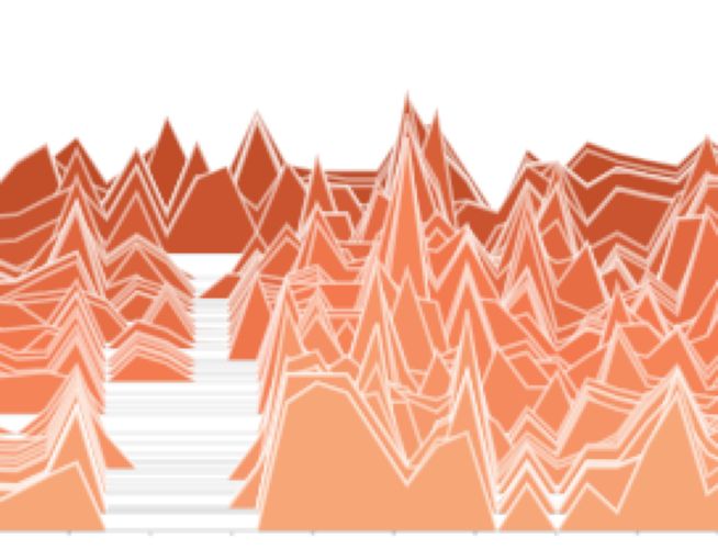
Under review as a conference paper at ICLR 2021

3.2   T RAINING

The proposed particle-based policy distribution is general and can be applied directly to any algo-
rithm using the policy gradient method with Equation 2. To initialize the training, due to lack of
prior knowledge, the particles can be distributed uniformly along the action dimensions with a stan-
dard deviation covering the gap between two successive particles. With no loss of generality, let us
consider below only one action dimension and drop the subscript k. Then, at every training step,
each particle i will move along its action dimension and be updated by
                                         "                                     #
                                           X
                           ∇J(φi ) = E        ct wi (st |θ)∇φi pi (at |φi )|st                   (4)
                                              t

where at ∼            is the action chosen during sampling, and ct = P wj (st A
             πθP (·|st )                                                        |θ)pj (at |φj ) is a coeffi-
                                                                                  t
                                                                              j
cient shared by all particles on the same action dimension. Our approach focuses only on the action
policy representation in general policy gradient methods. The estimation of At can be chosen as
required by the underlying policy gradient method, e.g. the generalized advantage estimator (Schul-
man et al., 2015b) in PPO/DPPO and the V-trace based temporal difference error in IMPALA.
Similarly, for the update of the policy neural network, we have
                                         "                                   #
                                           X
                            ∇J(θ) = E         ct pi (at |φi )∇θ wi (st |θ)|st .                         (5)
                                             t

From the above equations, although sampling is performed on only one particle for each given
dimension, all of that dimension’s particles will be updated during each training iteration to move
towards or away from the location of at according to At . The amount of the update, however, is
regulated by the state-dependent weight wi (st |θ): particles that have small probabilities to be chosen
for a given state st will be considered as uninteresting and be updated with a smaller step size or not
be updated at all. On the other hand, the contribution of weights is limited by the distance between a
particle and the sampled action: particles too far away from the sampled action would be considered
as insignificant to merit any weight gain or loss. In summary, particles can converge to different
optimal locations near them during training and be distributed multimodally according to the reward
landscape defined by At , rather than collapsing to a unimodal, Gaussian-like distribution.

3.3   R ESAMPLING

Similar to traditional particle filtering approaches, our approach would encounter the problem of
degeneracy (Kong et al., 1994). During training, a particle placed near a location at which sampling
gives a low At value would achieve a weight decrease. Once the associated weight reaches near
zero, the particle will not be updated anymore (cf. Equation 4) and become ‘dead’. We adapt the
idea of importance resampling from the particle filtering literature (Doucet et al., 2001) to perform
resampling for dead particles and reactivate them by duplicating alive target particles.
We consider a particle dead if its maximum weight over all possible states is too small, i.e.
maxst wi (st |θ) < , where  is a small positive threshold number. In practice, we cannot check
wi (st |θ) for all possible states, but can keep tracking it during sampling based on the observed
states collected in the last batch of environment steps. A target particle τi is drawn for each dead
particle i independently from the categorical distribution based on the particle’s average weight over
the observed samples: τi ∼ P (·|Est [wk (st |θ)] , k = 1, 2, · · · ).
Theorem 1. Let Dτ be a set of dead particles sharing the same target particle τ . Let also the
logits for the weight of each particle k be generated by a fully-connected layer with parameters
ωk for the weight and bk for the bias. The policy πθP (at |st ) is guaranteed to remain unchanged
after resampling via duplicating φi ← φτ , ∀i ∈ Dτ , if the weight and bias used to generate the
unnormalized logits of the target particle are shared with those of the dead one as follows:
                              ωi ← ωτ ;     bi , bτ ← bτ − log (|Dτ | + 1) .                            (6)
Proof. See Appendix B for the inference.
Theorem 1 guarantees the correctness of our resampling process as it keep the action policy
πθP (at |st ) identical before and after resampling. If, however, two particles are exactly the same

                                                     4
Under review as a conference paper at ICLR 2021

after resampling, they will always be updated together at the same pace during training and lose di-
versity. To address this issue, we add some regularization noise to the mean value when performing
resampling, i.e. µi ← µτ + εi , where εi is a small random number to prevent µi from being too
close to its target µτ .

3.4   R EPARAMETERIZATION T RICK

The two-step sampling method described in Section 3.1 is non-reparameterizable, because of the
standard way of sampling from the categorical distribution through which Gaussians are mixed. To
address this issue and enable the proposed action policy applicable in state-action value based off-
policy algorithms, we consider the concrete distribution (Jang et al., 2016; Maddison et al., 2016)
that generates a reparameterized continuous approximation to a categorical distribution. We refer to
Appendix D for a formal definition of concrete distribution defined as C ONCRETE below.
Let x(st |θ) ∼ C ONCRETE({wi (st |θ); i = 1, 2, · · · }, 1), where x(st |θ) = {xi (st |θ); i = 1, 2, · · · }
is a is a reparametrizable sampling result of a relaxed version of the one-hot categorical distribution
supported by the probability of {wi (st |θ); i = 1, 2, · · · }. We apply the Gumbel-softmax trick (Jang
et al., 2017) to get a sampled action value as
                                                                             !
                                               X
                            a0 (st ) = STOP       ai δ(i, arg max x(st |θ))                             (7)
                                                i

where ai is the sample drawn from the distribution represented by the particle i with parameter φi ,
STOP (·) is a “gradient stop” operation, and δ(·, ·) denotes the Kronecker delta function. Then, the
reparameterized sampling result can be written as follows:
                             X
                  aP
                   θ (st ) =    (ai − a0 (st ))mi + a0 (st )δ(i, arg max x) ≡ a0 (st ),          (8)
                               i

where mi := xi (st |θ) + STOP(δ(i, arg max x(st |θ)) − xi (st |θ)) ≡ δ(i, arg max x(st |θ)) com-
posing a one-hot vector that approximates the samples drawn from the corresponding categorical
distribution. Since xi (st |θ) drawn from the concrete distribution is differentiable to the parameter
θ, the gradient of the reparameterized action sample can be obtained by
                         X
          ∇θ a P
               θ (st ) =    (ai − a0 (st ))∇θ xi (st |θ); ∇φi aP
                                                               θ = δ(i, arg max x(st |θ))∇φi ai .  (9)
                         i

Through these equations, both the policy network parameter θ and the particle parameters φi can be
updated by backpropagation through the sampled action a0 (st ).

4     R ELATED W ORK
Our approach focuses on the action policy representation exploiting a more expressive distribution
other than Gaussians for continuous control problem in DRL using policy gradient method. In on-
policy gradient methods, action space discretization using a categorical distribution to replace the
original, continuous one has been successfully applied in some control tasks (Andrychowicz et al.,
2020; Tang & Agrawal, 2019). All of these works discretize the action space uniformly and convert
the action space to a discrete one before training. While impressive results have been obtained that
allow for better performance, such a uniform discretization scheme heavily relies on the number
of discretized atomic actions to find a good solution. On the other hand, discretized action spaces
cannot be directly applied on many off-policy policy gradient methods, since categorical distribu-
tions are non-reparameterizable. While DQN-like approaches are efficient for problems with dis-
crete action spaces, such techniques without policy networks cannot scale well to high-dimensional
continuous action spaces due to the curse of dimensionality (Lillicrap et al., 2015). Recent work
attempted to solve this issue by using a sequential model, at the expense, though, of increasing the
complexity of the state space (Metz et al., 2017). Chou et al. (2017) proposed to use beta distribu-
tions as a replacement to Gaussians. However, results from Tang & Agrawal (2018a) show that beta
distributions do not work well as Gaussians in high-dimensional tasks.
Our PFPN approach adopts a mixture distribution as the action policy, which becomes a mixture
of Gaussians when a learnable standard deviation variable is introduced to generate a normal noise

                                                     5
Under review as a conference paper at ICLR 2021

                                      AntBulletEnv-v0                             HumanoidBulletEnv-v0                                 DeepMimicWalk                                          DeepMimicPunch

Cumulative Rewards
                                PPO                                             DPPO                               600       DPPO                                         600       DPPO
                     3000                                            3000
                                                                                                                   400                                                    400
                     2000                                            2000
                                                 PFPN                                                              200                                                    200
                     1000                        Gaussian            1000
                                                 DISCRETE                                                            0                                                      0
                        0                                               0
                            0           1         2              3          0          1         2          3        0.0                0.5           1.0          1.5      0.0           0.5         1.0       1.5          2.0
                                       # of Samples        ×106                        # of Samples      ×107                          # of Samples             ×107                           # of Samples               ×107

Figure 1: Learning curves of PPO/DPPO using PFPN (blue) compared to Gaussian policies (red)
and DISCRETE policies (green). Solid lines report the average and shaded regions are the minimum
and maximum cumulative rewards achieved with different random seeds during training.

                                      AntBulletEnv-v0                             HumanoidBulletEnv-v0                                 DeepMimicWalk                                          DeepMimicPunch
Cumulative Rewards

                                SAC                                             SAC                                600       SAC                                          600       SAC
                     3000                                            3000
                                                                                                                   400                                                    400
                     2000                                            2000
                                                                                                                   200                                                    200
                     1000                             PFPN           1000
                                                      Gaussian                                                       0                                                      0
                        0                                               0
                            0           1         2              3          0           1        2             3         0         1          2   3         4         5         0         1       2         3         4      5
                                                                 6                                             7                                                      6
                                       # of Samples        ×10                         # of Samples      ×10                            # of Samples            ×10                             # of Samples              ×106

Figure 2: Comparison of SAC using PFPN (blue) and Gaussian policies (red). DISCRETE is not
shown as the categorical distribution cannot be applied to SAC.

for sampling. It uses state-independent particles having state-dependent weights to track the pol-
icy distribution. While an early version of SAC also employed a mixture of Gaussians, such a
mixture is completely state dependent, and hence it cannot provide a discretization scheme that is
consistent globally for all given states. In addition, the components in the fully state-dependent mix-
ture of Gaussians could collapse, resulting in similar issues as unimodal Gaussian policies (Tang
& Agrawal, 2018a). Adopting state-independent components can reduce the network size and still
provide expressive action policies when sufficient components are employed.
PFPN focuses on the policy distribution representation generated directly by the policy network
without changing the underlying policy gradient algorithms or remodeling the problem, and thus it
can be applied directly to most common used policy gradient methods in DRL. It is also comple-
mentary to recent works that focus on improving the expressiveness of the action policy through
normalizing flows (Haarnoja et al., 2018a; Tang & Agrawal, 2018b; Mazoure et al., 2019; Delal-
leau et al., 2019), where the mixture distribution provided by PFPN can be employed as a base
distribution. Other techniques applicable to policy gradient methods with a generally defined ba-
sic action policy can be combined with PFPN as well, such as the use of ordinal architecture for
action parameterization (Tang & Agrawal, 2019), action space momentum as in the recent PPO-
CMA (Hämäläinen et al., 2018), and energy-based policy distribution optimization methods, like
PGQL (O’Donoghue et al., 2016), Soft-Q learning (Haarnoja et al., 2017), SVPG (Liu et al., 2017),
and policy optimization using Wasserstein Gradient Flows (Zhang et al., 2018).

5                           E XPERIMENTS

The goal of our experiments is to evaluate whether existing policy gradient algorithms using PFPN
can outperform the corresponding implementations with Gaussian policies, along with comparing
our adaptive action discretization scheme generated by PFPN to the fixed, uniform one. For our
comparisons, we use the set of particles as a mixture of Gaussians with learnable standard deviation.
We run benchmarks on a range of continuous torque-based control tasks from PyBullet Roboschool
environments (Schulman et al., 2015a). We also consider several challenging position-control tasks
from the DeepMimic framework (Peng et al., 2018) where a 36-dimension humanoid agent learns a
locomotion policy based on motion capture data with a 197-dimension state space.

                                                                                                            6
Under review as a conference paper at ICLR 2021

5.1      C OMPARISONS

Figure 1 and 2 evaluate our approach on two representative policy gradient methods: PPO/DPPO
(Schulman et al., 2017; Heess et al., 2017), which is a stable on-policy method that exhibits good
performance, and SAC (Haarnoja et al., 2018d), an off-policy method that achieves state-of-the-art
performance in many tasks. The figures show the learning curve by cumulative rewards of evaluation
rollouts during training. We also compare PFPN to the fixed discretization scheme (DISCRETE)
obtained by uniformly discretizing each action dimension into a fixed number of bins and sampling
actions from a categorical distribution. In all comparisons, PFPN and DISCRETE exploit the same
number of atomic actions, i.e., number of particles in PFPN and number of bins in DISCRETE. We
train five trials of each baseline with different random seeds that are the same across PFPN and the
corresponding implementations of other methods. Evaluation was performed ten times every 1,000
training steps using deterministic action.
As it can be seen in Figure 1, PFPN outperforms Gaussian policies and DISCRETE in all of these
tested tasks. Compared to Gaussian policies, our particle-based scheme achieves better final perfor-
mance and typically exhibits faster convergence while being more stable across multiple trials. In
the Roboschool tasks, DISCRETE performs better than the Gaussian policies. However, this doesn’t
translate to the DeepMimic tasks where fine control demand is needed to reach DeepMimic’s mul-
timodal reward landscape, with DISCRETE showing high variance and an asymptotic performance
that is on par with or worse than Gaussian-based policies. In contrast, PFPN is considerably faster
and can reach stable performance that is higher than both Gaussian and DISCRETE policies.
In the SAC benchmarks shown in Figure 2, DISCRETE cannot be applied since the categorical
distribution that it employs as the action policy is non-parameterizable. PFPN works by exploiting
the reparameterization trick detailed in Section 3.4. Given the state-of-the-art performance of SAC,
the PFPN version of SAC performs comparably to or better than the vanilla SAC baseline and has
faster convergence in most of those tasks, which demonstrates the effectiveness of our proposed
adaptive discretization scheme. In DeepMimic tasks, considering the computation cost of running
stable PD controllers to determine the torque applied to each humanoid joint (Tan et al., 2011),
PFPN can save hours of training time due to its sampling efficiency.
PFPN can be applied to currently popular policy-gradient DRL algorithms. We refer to Appendix H
for additional benchmark results, as well as results obtained with A2C/A3C (Mnih et al., 2016),
IMPALA (Espeholt et al., 2018), and DDPG (Lillicrap et al., 2015). In most of these benchmarks,
PFPN outperforms the Gaussian baselines and DISCRETE scheme, and is more stable achieving
similar performance across different training trials. In Appendix H.5, we also compare the perfor-
mance in terms of wall clock time, highlighting the sampling efficiency of PFPN over Gaussian and
DISCRETE when facing complex control tasks. See Appendix G for all hyperparameters.

5.2      A DAPTIVE D ISCRETIZATION

 particles/         AntBulletEnv-v0           HumanoidBulletEnv-v0         DeepMimicWalk          DeepMimicPunch
   bins          PFPN          DISCRETE      PFPN           DISCRETE     PFPN      DISCRETE     PFPN       DISCRETE
    5         3154 ± 209     2958 ± 147   2568 ± 293     2567 ± 416    438 ± 15     61 ± 96    37 ± 15      10 ± 1
    10        3163 ± 323     2863 ± 281   2840 ± 480     2351 ± 343    489 ± 16    308 ± 86   426 ± 48    281 ± 155
    35        2597 ± 246     2367 ± 274   2276 ± 293     2255 ± 376     584 ± 4   245 ± 164    537 ± 7     317 ± 76
    50        2571 ± 163     2310 ± 239   2191 ± 322     1983 ± 325     580 ± 6   322 ± 195   521 ± 19    198 ± 159
   100        2234 ± 104     2181 ± 175   1444 ± 330     1427 ± 358    579 ± 18   277 ± 197    533 ± 7    224 ± 164
   150        2335 ± 147     2114 ± 160   1164 ± 323     1084 ± 453    583 ± 13   294 ± 200   531 ± 17    180 ± 152
   200                    -                           -                583 ± 15   360 ± 166   509 ± 31    181 ± 153
   400                    -                           -                578 ± 14   111 ± 159   478 ± 63    126 ± 137
 Gaussian            2327 ± 199                  2462 ± 195                  540 ± 19               359 ± 181

Table 1: Comparison between PFPN and DISCRETE on four benchmarks using PPO/DPPO while
varying the resolution of each action dimension.Training stops when a fixed number of samples is
met as shown in Figure 1. Reported numbers denote final performance averaged over 5 trials ± std.

Compared to Gaussian-based policy networks, DISCRETE can work quite well in many on-policy
tasks, as has been shown in recent prior work (Tang & Agrawal, 2019). However, in the comparative
evaluations outlined above, we showed that the adaptive discretization scheme that PFPN employs
results in higher asymptotic performance and/or faster convergence as compared to the uniform
discretization scheme. To gain a better understanding of the advantages of adaptive discretization

                                                            7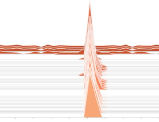
Under review as a conference paper at ICLR 2021

               X Axis                               Y Axis                               Z Axis                               Angle
                                                                                                                                                                       0

                                                                                                                                                      Training Steps
                                                                                                                                                                       1.5e7
-1.0   -0.6   -0.2   0.2   0.6   1.0 -1.0   -0.6   -0.2   0.2   0.6   1.0 -1.0   -0.6   -0.2   0.2   0.6   1.0 -1.0   -0.6   -0.2   0.2   0.6   1.0

Figure 3: Evolution of how particles are distributed along four action dimensions during training
of the DeepMimicWalk task with DPPO. The depicted four dimensions represent the target right
hip joint position expressed in an axis-angle representation. Each action dimension is normalized
between -1 and 1. Particles are initially distributed uniformly along a dimension (dark colors) and
their locations adaptively change as the policy network is trained (light colors). The training steps
are measured by the number of samples exploited during training.

for learning motor tasks, Table 1 further compares the performance of PFPN and DISCRETE across
different discretization resolutions (number of particles and number of bins, respectively). As it can
be seen, PFPN performs better than DISCRETE for any given resolution.
Intuitively, increasing the resolution, and hence the number of atomic actions, helps both DIS-
CRETE and PFPN. However, the more atomic actions employed the harder the optimization problem
will be for both methods due to the increase of policy gradient variance (see Appendix D for theo-
retical analysis). This can also be verified empirically by the performance decrease in Roboschool
tasks when transitioning from 10 to 150 particles. In the more complex DeepMimic tasks, using too
few atomic actions can easily skip over optimal actions. Although performance improves when the
action resolution increases from 5 to 10, DISCRETE cannot provide any stable training results as
denoted by the high variance among different trials. In contrast, PFPN performs significantly better
across all resolutions and can reach best performance using only 35 particles. And as the number of
particles increases beyond 35, PFPN has only a slight decrease in performance. This is because the
training of DeepMimic tasks was run long enough to ensure that it could reach a relatively stable
final performance. We refer to Appendix I for the sensitivity analysis of PFPN with respect to the
number of particles, where employing more atomic actions beyond the optimal number results in
slower convergence but similar final performance.
DeepMimic tasks rely on stable PD controllers and exploit motion capture data to design the re-
ward function, which is more subtle than the Roboschool reward functions that primarily measure
performance based on the torque cost and agent moving speed. Given a certain clip of motion, the
valid movement of a joint may be restrained in some small ranges, while the action space covers the
entire movement range of that joint. This makes position-based control problems more sensitive to
the placement of atomic actions, compared to Roboschool torque-based control tasks in which the
effective actions (torques) may be distributed in a relatively wide range over the action space. While
uniform discretization could place many atomic actions blindly in bad regions, PFPN optimizes the
placement of atomic actions, providing a more effective discretization scheme that reaches better
performance with fewer atomic actions. As an example, Figure 3 shows how particles evolve during
training for one of the humanoid’s joints in the DeepMimicWalk task where PFPN reaches a cumu-
lative imitation reward much higher than DISCRETE or Gaussian. We can see that the final active
action spaces cover only some small parts of the entire action space. In Appendix H, we also show
the particle evolution results for Roboschool’s AntBulletEnv-v0 task. Here, the active action spaces
are distributed more uniformly across the entire action space, which explains why DISCRETE is
able to exploit its atomic actions more efficiently than in DeepMimic tasks.

5.3      C ONTROL Q UALITY

To highlight the control performance of the adaptive discretization scheme, Figure 4 compares the
motion generated by PFPN and DISCRETE in the DeepMimicWalk task. As can be seen in the
figure, PFPN generates a stable motion sequence with a nature human-like gait, while DISCRETE
is stuck at a suboptimal solution and generates a walking motion sequence with an antalgic-like gait
where the agent walks forward mainly through the use of its left leg. From the motion trajectories,

                                                                             8
Under review as a conference paper at ICLR 2021

                                                                         Left Foot        Right Foot

 PFPN

                                                                                                        Left Foot
                                                                                                        Right Foot
 DISCRETE

                                                                                                       Left Foot
                                                                                                       Right Foot

Figure 4: Comparison of motion generated by PFPN and DISCRETE in DeepMimicWalk task
during one step cycle. Both PFPN and DISCRETE are trained with DPPO using the best resolution
parameters from Table 1 (35 particles and 200 bins, respectively). PCA embedding of the trajectories
of the agent’s two feet are shown at the right and their time sequence expansions at the bottom of
each method. Lines with “×” are the ground truth trajectories extracted from the motion capture
data that the agent learns to imitate.

                                                 Task        Force Direction PFPN DISCRETE  Gaussian
it can also be seen that PFPN results
                                                                Forward       588    340      512
in a more stable gait with a clear          DeepMimicWalk
                                                                Sideway       602    420      560
cyclic pattern strictly following the                           Forward      1156    480      720
motion capture data. We also assess         DeepMimicPunch
                                                                Sideway       896    576      748
the robustness of the learned poli-
cies to external perturbations. Table 2 Table 2: Minimal forwards and sideways push needed to
reports the minimal force needed make a DPPO DeepMimic agent fall down. Push force is in
to push the humanoid agent down. Newtons (N ) and applied on the chest of the agent for 0.1s.
All experiments were performed af-
ter training using deterministic actions. It is evident that the PFPN agent can tolerate much higher
forces than the Gaussian one. The fixed discretization in DISCRETE is less flexible, and as a result it
cannot learn generalized features that will enable robust agent control. We also refer to Appendix H
for additional results including motion trajectories obtained in the AntBulletEnv-v0 task, as well as
the controls (torque profiles) of the corresponding ant agents.

6           C ONCLUSION

We present a general framework for learning controls in high-dimensional continuous action spaces
through particle-based adaptive discretization. Our approach uses a mixture distribution represented
by a set of weighted particles to track the action policy using atomic actions during training. By
introducing the reparameterization trick, the resulting particle-based policy can be adopted by both
on-policy and off-policy policy gradient DRL algorithms. Our method does not change the underly-
ing architecture or learning mechanism of the algorithms, and is applicable to common actor-critic
policy gradient DRL algorithms. Overall, our particle filtering policy network combined with ex-
isting baselines leads to better performance and sampling efficiency as compared to corresponding
implementations with Gaussian policies. As a way to discretize the action space, we show that our
method is more friendly to policy gradient optimization by adaptive discretization, compared to uni-
form discretization, as it can optimize the placement of atomic actions and has the potential to meet
the fine control requirement by exploiting fewer atomic actions. In addition, it leads to high quality
motion and more robust agent control. While we currently track each action dimension indepen-
dently, accounting for the synergy that exists between different joints has the potential to further
improve performance and motion robustness, which opens an exciting avenue for future work.

                                                  9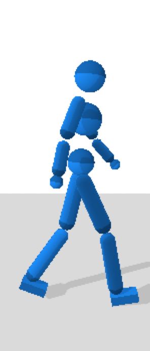
Under review as a conference paper at ICLR 2021

R EFERENCES
OpenAI: Marcin Andrychowicz, Bowen Baker, Maciek Chociej, Rafal Jozefowicz, Bob McGrew,
  Jakub Pachocki, Arthur Petron, Matthias Plappert, Glenn Powell, Alex Ray, et al. Learning
  dexterous in-hand manipulation. The International Journal of Robotics Research, 39(1):3–20,
  2020.
Po-Wei Chou, Daniel Maturana, and Sebastian Scherer. Improving stochastic policy gradients in
  continuous control with deep reinforcement learning using the beta distribution. In International
  conference on machine learning, pp. 834–843, 2017.
Erwin Coumans and Yunfei Bai. Pybullet, a python module for physics simulation for games,
  robotics and machine learning. http://pybullet.org, 2016–2019.
Christian Daniel, Gerhard Neumann, and Jan Peters. Hierarchical relative entropy policy search. In
  Artificial Intelligence and Statistics, pp. 273–281, 2012.
Olivier Delalleau, Maxim Peter, Eloi Alonso, and Adrien Logut. Discrete and continuous action
  representation for practical rl in video games. arXiv preprint arXiv:1912.11077, 2019.
Arnaud Doucet, Nando De Freitas, and Neil Gordon. An introduction to sequential monte carlo
  methods. In Sequential Monte Carlo methods in practice, pp. 3–14. Springer, 2001.
Lasse Espeholt, Hubert Soyer, Remi Munos, Karen Simonyan, Volodymir Mnih, Tom Ward, Yotam
  Doron, Vlad Firoiu, Tim Harley, Iain Dunning, et al. Impala: Scalable distributed deep-rl with
  importance weighted actor-learner architectures. arXiv preprint arXiv:1802.01561, 2018.
Scott Fujimoto, Herke Van Hoof, and David Meger. Addressing function approximation error in
  actor-critic methods. arXiv preprint arXiv:1802.09477, 2018.
Tuomas Haarnoja, Haoran Tang, Pieter Abbeel, and Sergey Levine. Reinforcement learning with
  deep energy-based policies. In International Conference on Machine Learning, pp. 1352–1361,
  2017.
Tuomas Haarnoja, Kristian Hartikainen, Pieter Abbeel, and Sergey Levine. Latent space policies for
  hierarchical reinforcement learning. arXiv preprint arXiv:1804.02808, 2018a.
Tuomas Haarnoja, Aurick Zhou, Pieter Abbeel, and Sergey Levine. Soft actor-critic: Off-
  policy maximum entropy deep reinforcement learning with a stochastic actor. arXiv preprint
  arXiv:1801.01290, 2018b.
Tuomas Haarnoja, Aurick Zhou, Sehoon Ha, Jie Tan, George Tucker, and Sergey Levine. Learning
  to walk via deep reinforcement learning. In Robotics: Science and Systems, 2018c.
Tuomas Haarnoja, Aurick Zhou, Kristian Hartikainen, George Tucker, Sehoon Ha, Jie Tan, Vikash
  Kumar, Henry Zhu, Abhishek Gupta, Pieter Abbeel, et al. Soft actor-critic algorithms and appli-
  cations. arXiv preprint arXiv:1812.05905, 2018d.
Perttu Hämäläinen, Amin Babadi, Xiaoxiao Ma, and Jaakko Lehtinen. Ppo-cma: Proximal policy
  optimization with covariance matrix adaptation. arXiv preprint arXiv:1810.02541, 2018.
Nicolas Heess, Srinivasan Sriram, Jay Lemmon, Josh Merel, Greg Wayne, Yuval Tassa, Tom Erez,
  Ziyu Wang, SM Eslami, Martin Riedmiller, et al. Emergence of locomotion behaviours in rich
  environments. arXiv preprint arXiv:1707.02286, 2017.
Marco F Huber, Tim Bailey, Hugh Durrant-Whyte, and Uwe D Hanebeck. On entropy approxima-
 tion for gaussian mixture random vectors. In 2008 IEEE International Conference on Multisensor
 Fusion and Integration for Intelligent Systems, pp. 181–188. IEEE, 2008.
Eric Jang, Shixiang Gu, and Ben Poole. Categorical reparameterization with gumbel-softmax. arXiv
  preprint arXiv:1611.01144, 2016.
Eric Jang, Shixiang Gu, and Ben Poole. Categorical reparametrization with gumble-softmax. In
  International Conference on Learning Representations (ICLR 2017), 2017.

                                                10
Under review as a conference paper at ICLR 2021
Wojciech Jaśkowski, Odd Rune Lykkebø, Nihat Engin Toklu, Florian Trifterer, Zdeněk Buk, Jan
Koutnı́k, and Faustino Gomez. Reinforcement learning to run. . . fast. In The NIPS’17 Competi-
tion: Building Intelligent Systems, pp. 155–167. Springer, 2018.
Diederik P Kingma and Jimmy Ba. Adam: A method for stochastic optimization. arXiv preprint
arXiv:1412.6980, 2014.
Augustine Kong, Jun S Liu, and Wing Hung Wong. Sequential imputations and bayesian missing
data problems. Journal of the American statistical association, 89(425):278–288, 1994.
Sergey Levine, Chelsea Finn, Trevor Darrell, and Pieter Abbeel. End-to-end training of deep visuo-
motor policies. The Journal of Machine Learning Research, 17(1):1334–1373, 2016.
Timothy P Lillicrap, Jonathan J Hunt, Alexander Pritzel, Nicolas Heess, Tom Erez, Yuval Tassa,
David Silver, and Daan Wierstra. Continuous control with deep reinforcement learning. arXiv
preprint arXiv:1509.02971, 2015.
Yang Liu, Prajit Ramachandran, Qiang Liu, and Jian Peng. Stein variational policy gradient. arXiv
preprint arXiv:1704.02399, 2017.
Chris J Maddison, Andriy Mnih, and Yee Whye Teh. The concrete distribution: A continuous
relaxation of discrete random variables. arXiv preprint arXiv:1611.00712, 2016.
Bogdan Mazoure, Thang Doan, Audrey Durand, R Devon Hjelm, and Joelle Pineau. Leveraging
exploration in off-policy algorithms via normalizing flows. arXiv preprint arXiv:1905.06893,
2019.
Luke Metz, Julian Ibarz, Navdeep Jaitly, and James Davidson. Discrete sequential prediction of
continuous actions for deep rl. arXiv preprint arXiv:1705.05035, 2017.
Volodymyr Mnih, Adria Puigdomenech Badia, Mehdi Mirza, Alex Graves, Timothy Lillicrap, Tim
Harley, David Silver, and Koray Kavukcuoglu. Asynchronous methods for deep reinforcement
learning. In International conference on machine learning, pp. 1928–1937, 2016.
Rémi Munos, Tom Stepleton, Anna Harutyunyan, and Marc Bellemare. Safe and efficient off-policy
reinforcement learning. In Advances in Neural Information Processing Systems, pp. 1054–1062,
2016.
Ofir Nachum, Mohammad Norouzi, Kelvin Xu, and Dale Schuurmans. Bridging the gap between
value and policy based reinforcement learning. In Advances in Neural Information Processing
Systems, pp. 2775–2785, 2017.
Brendan O’Donoghue, Remi Munos, Koray Kavukcuoglu, and Volodymyr Mnih. Combining policy
gradient and q-learning. arXiv preprint arXiv:1611.01626, 2016.
George Papandreou and Alan L Yuille. Perturb-and-map random fields: Using discrete optimization
to learn and sample from energy models. In 2011 International Conference on Computer Vision,
pp. 193–200. IEEE, 2011.
Xue Bin Peng, Pieter Abbeel, Sergey Levine, and Michiel van de Panne. Deepmimic: Example-
guided deep reinforcement learning of physics-based character skills. ACM Transactions on
Graphics (TOG), 37(4):1–14, 2018.
Xue Bin Peng, Erwin Coumans, Tingnan Zhang, Tsang-Wei Lee, Jie Tan, and Sergey Levine. Learn-
ing Agile Robotic Locomotion Skills by Imitating Animals. In Proceedings of Robotics: Science
and Systems, 2020.
Aravind Rajeswaran, Vikash Kumar, Abhishek Gupta, Giulia Vezzani, John Schulman, Emanuel
Todorov, and Sergey Levine. Learning complex dexterous manipulation with deep reinforcement
learning and demonstrations. In Robotics: Science and Systems, 2018.
Andrew M Saxe, James L McClelland, and Surya Ganguli. Exact solutions to the nonlinear dynam-
ics of learning in deep linear neural networks. arXiv preprint arXiv:1312.6120, 2013.
11Under review as a conference paper at ICLR 2021
John Schulman, Sergey Levine, Pieter Abbeel, Michael Jordan, and Philipp Moritz. Trust region
policy optimization. In International conference on machine learning, pp. 1889–1897, 2015a.
John Schulman, Philipp Moritz, Sergey Levine, Michael Jordan, and Pieter Abbeel. High-
dimensional continuous control using generalized advantage estimation. arXiv preprint
arXiv:1506.02438, 2015b.
John Schulman, Filip Wolski, Prafulla Dhariwal, Alec Radford, and Oleg Klimov. Proximal policy
optimization algorithms. arXiv preprint arXiv:1707.06347, 2017.
Richard S Sutton, David A McAllester, Satinder P Singh, and Yishay Mansour. Policy gradient
methods for reinforcement learning with function approximation. In Advances in neural informa-
tion processing systems, pp. 1057–1063, 2000.
Jie Tan, Karen Liu, and Greg Turk. Stable proportional-derivative controllers. IEEE Computer
Graphics and Applications, 31(4):34–44, 2011.
Jie Tan, Tingnan Zhang, Erwin Coumans, Atil Iscen, Yunfei Bai, Danijar Hafner, Steven Bohez, and
Vincent Vanhoucke. Sim-to-real: Learning agile locomotion for quadruped robots. In Robotics:
Science and Systems, 2018.
Yunhao Tang and Shipra Agrawal. Boosting trust region policy optimization by normalizing flows
policy. arXiv preprint arXiv:1809.10326, 2018a.
Yunhao Tang and Shipra Agrawal. Implicit policy for reinforcement learning. arXiv preprint
arXiv:1806.06798, 2018b.
Yunhao Tang and Shipra Agrawal. Discretizing continuous action space for on-policy optimization.
arXiv preprint arXiv:1901.10500, 2019.
Ruiyi Zhang, Changyou Chen, Chunyuan Li, and Lawrence Carin. Policy optimization as wasser-
stein gradient flows. arXiv preprint arXiv:1808.03030, 2018.
12Under review as a conference paper at ICLR 2021
A A LGORITHM
Algorithm 1 Policy Gradient Method using Particle Filtering Policy Network
Initialize the neural network parameter θ and learning rate α;
initialize particle parameters φi to uniformly distribute particles on the action dimension;
initialize the threshold to detect dead particles using a small number;
initialize the value of interval n to perform resampling.
loop
for each environment step do
// Record the weight while sampling.
at ∼ πθ,P (·|st )
Wi ← Wi ∪ {wi (st |θ)}
end for
for each training step do
// Update parameters using SGD method.
φi ← φi + α∇J(φi )
θ ← θ + α∇J(θ)
end for
for every n environment steps do
// Detect dead particles and set up target ones.
for each particle i do
if maxwi ∈Wi wi < then
τi ∼ P (·|E [wk |wk ∈ Wk ] , k = 1, 2, · · · )
T ← T ∪ {τi }; Dτi ← Dτi ∪ {i}
end if
end for
// Resampling.
for each target particle τ ∈ T do
for each dead particle i ∈ Dτ do
// Duplicate particles.
φi ← φτ with µi ← µτ + εi
// Duplicate parameters of the last layer in the policy network.
ωi ← ωτ ; bi ← bτ − log(|Dτ | + 1)
end for
bτ ← bτ − log(|Dτ | + 1)
Dτ ← ∅
end for
T ← ∅; Wi ← ∅
end for
end loop
B P OLICY N ETWORK L OGITS C ORRECTION DURING R ESAMPLING
Theorem 1. Let Dτ be a set of dead particles sharing the same target particle τ . Let also the
logits for the weight of each particle k be generated by a fully-connected layer with parameters
ωk for the weight and bk for the bias. The policy πθP (at |st ) is guaranteed to remain unchanged
after resampling via duplicating φi ← φτ , ∀i ∈ Dτ , if the weight and bias used to generate the
unnormalized logits of the target particle are shared with those of the dead one as follows:
ωi ← ωτ ; bi , bτ ← bτ − log (|Dτ | + 1) . (10)
Proof. The weight for the i-th particle is achieved by softmax operation, which is applied to the
unnormalized logits Li , i.e. the direct output of the policy network:
eLi (st )
wi (st ) = SOFTMAX(Li (st )) = P L (s ) . (11)
ke
k t
Resampling via duplicating makes dead particles become identical to their target particle. Namely,
particles in Dτ ∪ {τ } will share the same weights as well as the same value of logits, say L0τ , after
13Under review as a conference paper at ICLR 2021
resampling. To ensure the policy identical before and after sampling, the following equation must
be satisfied X X 0 X
eLk (st ) = eLτ (st ) + eLk (st ) (12)
k Dτ ∪{τ } k6∈Dτ ∪{τ }
where Lk is the unnormalized logits for the k-th particle such that the weights for all particles who
are not in Dτ ∪ {τ } unchanged, while particles in Dτ ∪ {τ } share the same weights.
A target particle will not be tagged as dead at all, i.e. τ 6∈ Dk for any dead particle set Dk , since
a target particle is drawn according to the particles’ weights and since dead particles are defined as
the ones having too small or zero weight to be chosen. Hence, Equation 12 can be rewritten as
X 0
eLi (st ) + eLτ (st ) = (|Dτ | + 1)eLτ (st ) , (13)
i∈Dτ
Given that eLi (st ) ≈ 0 for any dead particle i ∈ Dτ and that the number of particles is limited, it
implies that
0
eLτ ≈ (|Dτ | + 1)eLτ (st ) . (14)
Taking the logarithm of both sides of the equation leads to that for all particles in Dτ ∪ {τ }, their
new logits after resampling should satisfy
L0τ (st ) ≈ Lτ (st ) − log(|Dτ | + 1). (15)
Assuming the input of the full-connected layer who generates Li is x(st ), i.e. Li (st ) = ωi x(st )+bi ,
we have
ωi0 x(st ) + b0i = ωτ x(st ) + bτ − log (|Dτ | + 1) . (16)
Then, Theorem 1 can be reached.
If we perform random sampling not based on the weights during resampling (see Appendix I), it is
possible to pick a dead particle as the target particle. In that case
X
L0τ (st ) ≈ Lτ (st ) − log(|Dτ | + (1 − δ(τ, Dk ))), (17)
k
where L0τ (st ) is the new logits shared by particles in Dτ and δ(τ, Dk ) is the Kronecker delta function
1 if τ ∈ Dk
δ(τ, Dk ) = (18)
0 otherwise
P
that satisfies k δ(τ, Dk ) ≤ 1. Then, for the particle τ , its new logits can be defined as
X X
L00τ (st ) ≈ (1 − δ(τ, Dk ))L0τ (st ) + δ(τ, Dk )Lτ . (19)
k k
Consequently, the target particle τ may or may not share the same logits with those in Dτ , depending
on if it is tagged as dead or not.
C P OLICY R EPRESENTATION WITH ACTION B OUNDS
In off-policy algorithms, like DDPG and SAC, an invertible squashing function, typically the
hyperbolic tangent function, will be applied to enforce action bounds on samples drawn from
Gaussian distributions, e.g. in SAC, the action is obtained by at (ε, st ) = tanh ut,k where
ut,k ∼ N (µθ (st ), σθ2 (st )), and µθ (st ) and σθ2 (st )) are parameters generated by the policy network
with parameter θ.
Let at = {tanh ut,k } where ut,k , drawn from the distribution represented by a particle with pa-
rameter φt,k , is a random variable sampled to support the action on the k-th dimension. Then, the
probability density function of PFPN represented by Equation 3 can be rewritten as
YX
πθP (at |st ) = wi,k (st |θ)pi,k (ut,k |φi,k )/(1 − tanh2 ut,k ), (20)
k i
and the log-probability function becomes
" #
X X
P
log πθ (at |st ) = log wi,k (st |θ)pi,k (ut,k |φi,k ) − 2 (log 2 − ut,k − softplus(−2ut,k )) .
k i
(21)
14Under review as a conference paper at ICLR 2021
D C ONCRETE D ISTRIBUTION
Concrete distribution was introduced by Maddison et al. (2016). It is also called Gumbel-Softmax
and proposed by Jang et al. (2016) concurrently. Here, we directly give the definition of concrete
random variables X ∼ C ONCRETE(α, λ) by its density function using the notion from Maddison
et al. (2016) as below:
n
!
n−1
Y αk xk−λ−1
pα,λ (x) = (n − 1)!λ Pn −λ
, (22)
k=1 i=1 αi xi
Pn
where X ∈ {x ∈ Rn |xk ∈ [0, 1], k=1 xk = 1}, α = {α1 , · · · , αn } ∈ (0, +∞)n is the location
parameter and λ ∈ (0, +∞) is the temperature parameter. A sample X = {X1 , · · · , Xn } can be
drawn by
exp((log αk + Gk )/λ)
Xk = Pn , (23)
i=1 exp((log αi + Gi )/λ)
where Gk ∼ G UMBEL i.i.d., or more explicitly, Gk = − log(− log Uk ) with Uk drawn from
U NIFORM(0, 1).
From Equation 23, X can be reparameterized using the parameter α and λ, and gives us a relaxed
version of continuous approximation to the one-hot categorical distribution supported by the logits
α. As λ is smaller, the approximation is more discrete and accurate. In all of our experiments, we
pick λ = 1.
For convenience,
Pn in Section 3.4, we use C ONCRETE with parameter w ∈ {w1 , · · · , wn |wk ∈
[0, 1], k=1 wk = 1} as the probability weight to support a categorical distribution instead of the
logits α. We can get α in terms of w by
αk = log(wk /(1 − wk )). (24)
Since X ∼ C ONCRETE(α, λ) is a relaxed one-hot result, we use arg max X to decide which particle
to choose in the proposed reparameterization trick.
E VARIANCE OF P OLICY G RADIENT IN PFPN C ONFIGURATION
Since each action dimension is independent to others, without loss of generality, we here consider
the action at with only one dimension along which n particles are distributed and the particle i
to represent a Gaussian distribution N (µi , σi2 ). In order to make it easy for analysis, we set up
the following assumptions: the reward estimation is constant, i.e. At ≡ A; logits to support the
weights of particles are initialized equally, i.e. wi (st |θ) ≡ n1 for all particles i and ∇θ w1 (st |θ) =
· · · = ∇θ wn (st |θ); particles are initialized to equally cover the whole action space, i.e. µi = i−n n ,
2 1
σi ≈ n2 where i = 1, · · · , n.
From Equation 5, the variance of the policy gradient under such assumptions is
R At Pi pi (at |µt ,σt )∇θ wi (st |θ) 2
V[∇θ J(θ)|at ] = P at dat
i wi (st |θ)pi (at |µt ,σt )
∝ i ∇θ wi (st |θ) a2t pi (at |µt , σt )dat
P R
∝ 2
+ σi2 )∇θ wi (st |θ)
P
∼ i (µi
(25)
P (i−n)2 +1
∝ i n2
n 7 1
= 3 + 6n − 2
3
∼1− 2n + O( n12 ).
Given V[∇θ J(θ)|at ] = 0 when n = 1, from Equation 25, for any n > 0, the variance of policy
gradient V[∇J(θ)|at ] will increase with n. Though the assumptions usually are hard to meet per-
fectly in practice, this still gives us an insight that employing a large number of particles may result
in more challenge to optimization.
15You can also read