Adaptive Variable Step Size in LMS Algorithm Using Evolutionary Programming: VSSLMSEV
←
→
Page content transcription
If your browser does not render page correctly, please read the page content below
Ajjaiah H.B.M, P.V.Hunagund, Manoj Kumar Singh & P.V.Rao
Adaptive Variable Step Size in LMS Algorithm Using
Evolutionary Programming: VSSLMSEV
Ajjaiah H.B.M hbmajay@gmail.com
Research scholar
Jyothi institute of Technology
Bangalore, 560006, India
Prabhakar V Hunagund prabhakar_hunagund@yahoo.co.in
Dept.of PG atudies and Research in applied electronics
Jnana Ganga, Gulbarga University
Gulbarga - 585106, India
Manoj Kumar Singh mksingh@manuroresearch.com
Director
Manuro Tech Research
Bangalore, 560097, India
P.V.Rao pachararao@rediffmail.com
Dept.of ECE,RGIT,
Bangalore,India
Abstract
The Least Mean square (LMS) algorithm has been extensively used in many applications due to its
simplicity and robustness. In practical application of the LMS algorithm, a key parameter is the step
size. As the step size becomes large /small, the convergence rate of the LMS algorithm will be rapid
and the steady-state mean square error (MSE) will increase/decrease. Thus, the step size provides a
trade off between the convergence rate and the steady-state MSE of the LMS algorithm. An intuitive
way to improve the performance of the LMS algorithm is to make the step size variable rather than
fixed, that is, choose large step size values during the initial convergence of the LMS algorithm, and
use small step size values when the system is close to its steady state, which results invariable step
size Least Mean square (VSSLMS) algorithms. By utilizing such an approach, both a fast convergence
rate and a small steady-state MSE can be obtained. Although many VSSLMS algorithmic methods
perform well under certain conditions, noise can degrade their performance and having performance
sensitivity over parameter setting. In this paper, a new concept is introduced to vary the step size
based upon evolutionary programming (VSSLMSEV) algorithm is described. It has shown that the
performance generated by this method is robust and does not require any presetting of involved
parameters in solution based upon statistical characteristics of signal.
Keywords: Adaptive Equalization, LMS Algorithm, Step Size, Evolutionary Programming, MSE.
1. INTRODUCTION
The recent digital transmission systems impose the application of channel equalizers with short
training time and high tracking rate. These requirements turn our attention to adaptive algorithms,
which converge rapidly. One of the most important advantages of the digital transmission
systems for voice, data and video communications is their higher reliability in noise environment
in comparison with that of their analog counterparts. Unfortunately most often the digital
transmission of information is accompanied with a phenomenon known as intersymbol
interference (ISI). Briefly this means that the transmitted pulses are smeared out so that pulses
that correspond to different symbols are not separable. Depending on the transmission media the
main causes for ISI are: cable lines – the fact that they are band limited; cellular communications
– multipath propagation. Obviously for a reliable digital transmission system it is crucial to reduce
Signal Processing: An International Journal (SPIJ), Volume (6) : Issue (2) : 2012 78
Ajjaiah H.B.M, P.V.Hunagund, Manoj Kumar Singh & P.V.Rao

the effects of ISI and it is where the adaptive equalizers come on the scene. Two of the most
intensively developing areas of digital transmission, namely digital subscriber lines and cellular
communications are strongly dependent on the realization of reliable channel equalizers. One of
the possible solutions is the implementation of equalizer based on filter with finite impulse
response (FIR) employing the well known LMS algorithm for adjusting its coefficients. The LMS
algorithm is one of the most popular algorithms in adaptive signal processing. Due to its simplicity
and robustness, it has been the focus of much study and its implementation in many applications.
The popularity stems from its relatively low computational complexity, good numerical stability,
simple structure, and ease of implementation in terms of hardware. The essence of LMS
algorithm is to update the adaptive filter coefficients recursively along the negative gradient of
estimate error surface. Conventional algorithm uses a fixed step-size to perform the iteration, and
to get a compromise between the conflict of fast convergence and small steady-state MSE.A
small step-size could ensure small MSE with a slow convergence, where as a large step-size will
provide a faster convergence and better tracking capabilities at the cost of higher steady-state
MSE. Therefore, fixed step-size LMS algorithm definitely cannot settle this contradiction.
Consequently, many variable step-size algorithms were proposed to solve the problem. Though
these algorithms could accelerate convergence and deduce steady-state MSE to some extent,
they failed to analyze the optimality of variable step-size LMS further. LMS algorithm is described
by the following equations:

e (n) = d(n) - XT (n) * W (n)                 -------                     (1)
W (n + 1) = W (n) + µe(n) X(n)                -------                     (2)

where µ is learning step, X(n)is the input vector at sampling time n,W (n) is the coefficient vector
of the adaptive filter, d(n) is the expected output value e(n) is the deviation error, dimension of
W (n) is the length of the adaptive filter.

2    RELATED WORK
In this work we introduced a novel method to obtain an optimal step-size and an algorithm for
LMS. The algorithm runs iteratively and convergence to the equalizer coefficients by finding the
optimal step-size which minimizes the steady-state error rate at each iteration. No initialization for
the step-size value is required. Efficiency of the proposed algorithm is shown by making a
performance comparison between some of the other LMS based algorithms and optimal step-size
LMS algorithm [1].A variation of gradient adaptive step-size LMS algorithms are presented. They
propose a simplification to a class of the studied algorithms [2]. Adaption in the variable step size
LMS proposed by [3] based on weighting coefficients bias/variance trade off. Authors in [4]
examine the stability of VSLMS with uncorrelated stationary Gaussian data. Most VSLMS
described in the literature use a data-dependent step-size, where the step-size either depends on
the data before the current time (prior step-size rule) or through the current time (posterior step-
size rule).It has often been assumed that VSLMS algorithms are stable (in the sense of mean-
square bounded weights), provided that the step-size is constrained to lie within the
corresponding stability region for the LMS algorithm. The analysis of these VSLMS algorithms in
the literature typically proceeds in two steps [5], [6]. First, a rigorous stability analysis is
attempted, apparently leading to conditions for MSE bounded weights and bounded MSE, and
second, an approximate performance analysis is carried out, including convergence to and
characterization of the asymptotic weight mean, covariance, and MSE. Thus one can at least
guarantee stability (MS bounded weights) rigorously would seem to support the performance
analysis. Two methods of variable step-size normalized least mean square (NLMS) and affine
projection algorithms (APA) with variable smoothing factor have presented in [8]. With the
Simulation results they have illustrated that the proposed algorithms have improvement in
convergence rate and lower small adjustment error.

3. BASIC CRITERIA FOR PERFORMANCE
The performance of the LMS adaptive filter can be characterized in three important ways: i) the
adequacy of the FIR filter Model (ii) the speed of convergence of the system and iii) the small

Signal Processing: An International Journal (SPIJ), Volume (6) : Issue (2) : 2012                  79
Ajjaiah H.B.M, P.V.Hunagund, Manoj Kumar Singh & P.V.Rao

adjustment steady-state.

3.1 Speed of Convergence
The rate at which the coefficients approach their optimum values is called the speed of
convergence. As per the previous analytical result obtained, there exists no one quantity that
characterizes the speed of convergence, as it depends on the initial coefficient values, the
amplitude and correlation statistics of the signals, the filter length L, and the step size µ(n).

However, we can make several qualitative statements relating the speed of convergence to both
the step size and the filter length. All of these results assume that the desired response signal
model is reasonable and the errors in the filter coefficients are uniformly distributed across the
coefficients on average.

• The speed of convergence increases as the value of the step size is increased, up to step sizes
near one-half the maximum value required for stable operation of the system. This result can be
obtained from a careful analysis for different input signal types and correlation statistics. For
typical signal scenarios, it is observed that the speed of convergence of the excess MSE actually
decreases for large enough step size values.

• The maximum possible speed of convergence is limited by the largest step size that can be
chosen for stability for moderately correlated input signals. In practice, the actual step size
needed for stability of the LMS adaptive filter is smaller than one-half the maximum values when
the input signal is moderately correlated. This effect is due to the actual statistical relationships
between the current coefficient vector and the signals. Since the convergence speed increases
as µ is increased over this allowable step size range, the maximum stable step size provides a
practical limit on the speed of convergence of the system.

3.2 Choice of Step Size
Based on the previous result obtained, the speed of convergence as the step is increased. We
have seen that the speed of convergence increases as the step size is increased, up to values
that are roughly within a factor of 1/2 of the step size stability limits. Thus, if fast convergence is
desired, one should choose a large step size according to the limits. However, we also observe
that the small adjustment increases as the step size is increased. Therefore, if highly accurate
estimates of the filter coefficients are desired, a small step size should be chosen. This classical
trade off in convergence speed versus the level of error in steady state dominates the issue of
step size selection in many estimation schemes. If the user knows that the relationship between
input signal x(n) and desired signal d(n)is linear and time-invariant, then one possible solution to
the above trade off is to choose a large step size initially to obtain fast convergence, and then
switch to a smaller step size. The point to switch to a smaller step size is roughly when the
excess MSE becomes a small fraction (approximately 1/10th) of the minimum MSE of the filter.
This method of gear shifting, as it is commonly known, is part of a larger class of time-varying
step size methods.

4. EVOLUTIONARY COMPUTATION
Evolutionary algorithms are stochastic search methods that mimic the metaphor of natural
biological evolution. Evolutionary algorithms operate on a population of potential solutions
applying the principle of survival of the fittest to produce better and better approximations to a
solution. At each generation, a new set of approximations is created by the process of selecting
individuals according to their level of fitness in the problem domain and breeding them together
using operators borrowed from natural genetics. This process leads to the evolution of
populations of individuals that are better suited to their environment than the individuals that they
were created from, just as in natural adaptation. Evolutionary computation uses computational
models of evolutionary processes as key elements in the design and implementation of computer-
based problem solving systems. There are a variety of evolutionary computational models that
have been proposed and studied (evolutionary algorithms). They share a common conceptual

Signal Processing: An International Journal (SPIJ), Volume (6) : Issue (2) : 2012                   80
Ajjaiah H.B.M, P.V.Hunagund, Manoj Kumar Singh & P.V.Rao

base of simulating the evolution of individual structures via processes of selection and
reproduction. These processes depend on the perceived performance (fitness) of the individual
structures as defined by an environment. More precisely, evolutionary algorithms maintain a
population of structures that evolve according to rules of selection and other operators such as
recombination and mutation. Each individual in the population receives a measure of its fitness in
the environment. Selection focuses attention on high fitness individuals, thus exploiting the
available fitness information. Recombination and mutation perturb those individuals, providing
general heuristics for exploration. Although simplistic from a biologist’s viewpoint, these
algorithms are sufficiently complex to provide robust and powerful adaptive search mechanisms.

                                             Procedure EP; {
                                                t = 0;
                                              Initialize population P (t);
                                               Evaluate P (t);
                                                Until (done) {
                                                                                        t = t + 1;
                                                                     Parent selection P (t);
                                                                              Mutate P (t);
                                                                             Evaluate P (t);
                                                                             Survive P (t);

                                                                                    }   }

Evolutionary algorithms (EA) differ substantially from more traditional search and optimization
methods. The most significant differences of EA are:
• search a population of points in parallel, not just a single point.
• not require derivative information or other auxiliary knowledge; only the objective function
and corresponding fitness levels influence the directions of search.
• use probabilistic transition rules, not deterministic ones.
• generally more straightforward to apply, because no restrictions for the definition of the objective
function exist.
•Provide a number of potential solutions to a given problem. The final choice is left to the user.
(Thus, in cases where the particular problem does not have one individual solution, for example a
family of pareto-optimal solutions),as in the case of multi-objective optimization and scheduling
problems, then the evolutionary algorithm is potentially useful for identifying these alternative
solutions simultaneously.

4.1. Algorithmic View of EP in VSSLMSEV
Evolutionary programming (EP), developed by Fogel et al. traditionally has used representations
that are tailored to the problem domain. For example, in real valued optimization problems, the
individuals within the population are real-valued vectors. Similarly, ordered lists are used for
traveling salesman problems, and graphs for applications with finite state machines. EP is often
used as an optimizer, although it arose from the desire to generate machine intelligence. The
outline of the evolutionary programming algorithm is shown below

Signal Processing: An International Journal (SPIJ), Volume (6) : Issue (2) : 2012                    81
Ajjaiah H.B.M, P.V.Hunagund, Manoj Kumar Singh & P.V.Rao
(i). Generate initial population of µ individuals and set k=1, each individual is taken as a pair
of real valued vectors (pi, ηi ),∀ i={1,……μ}
(ii). Evaluate the fitness score of each individual (pi, ηi ),∀ i={1,……μ}
of the population based on the objective function.
(iii). Each parent (pi, ηi ),∀ i={1,……μ}creates a single offspring(pi’, ηi’ ) by:
p’i(j) = pi (j) + η i(j). N (0,1) -------------------(3)
η’i (j) = ηi (j) exp(τ’ N(0,1) + τ Nj(0,1)) -------------------(4)
for j=1…n.where N(0,1) is a Gaussian random variable with zero mean and unity standard
deviation and Nj(0,1) is generated a new for each value of j. pi (j), p’i (j), ηi (j), η’i (j)
,denote the jth component of vector pi, p’i, ηi, η’i respectively. The factor τ and τ’ are
commonly set to ( √(2√n) )-1 and ( √2n)-1 .
(iv). Calculate the fitness of each offspring (pi, ηi ),∀ i={1,……μ}
(v). From the union of parents (pi, ηi ) and offspring(pi, ηi ),∀ i={1,……μ} select the µ
individuals have the maximum fitness to be parents of the next generation
5. SIMULATION
To see the performance of EVSSLMS, for channel, number of taps selected for equalizer is
11istaken. Input signal contains total 500 samples generated randomly through uniform
distribution shown in fig1. Gaussian noise having zero mean and 0.01 standard deviation added
with input signal as shown in fig2.channel characteristics is given by the vector:
[0.05 -0.063 0.088 -0.126 -0.25 0.9047 0.25 0 0.126 0.038 0.088]
5.1 Case1: LMS with fixed step size
A rule of thumb available in number of literatures applied for selecting the step size in order to
ensure convergence and good tracking capability in slow varying channel.
∆=1/(5*(2K+1)*PR) --------------(5)
Where PR denotes the received signal plus noise power, which can be estimated from the
received signal .in the taken input signal value of ∆ from eq(5) is equal to 0.0088. Three different
value of fixed step size applied with LMS to see the difference in performance: (a) 0.11(b) 0.045
(c) 0.0088 and resulting performance has shown in the fig(3).form the result it is clear that it is
very difficult to find the optimal step size.
5.2 Case 2: LMS With Adaptive Variable Step Size
To over the problem of optimal step size evolutionary computation as given above applied. For
each iteration one generation created and fittest step size in that generation taken for that
particular iteration. From previous generation a new generation created by mutation process
defined in eq (3) and in eq (4), for next iteration and process will keep continue until all iteration
are not completed.
Parameter setting: Initial population is defined by uniform distribution random variable in the
range of [0 1] and ηi is taken as 0.000005,∀ i={1,2,…….µ} and fitness of solution is defined by
݂=1/MSE.
Signal Processing: An International Journal (SPIJ), Volume (6) : Issue (2) : 2012 82Ajjaiah H.B.M, P.V.Hunagund, Manoj Kumar Singh & P.V.Rao
FIGURE 1: generated input signal and signal with noise from channel
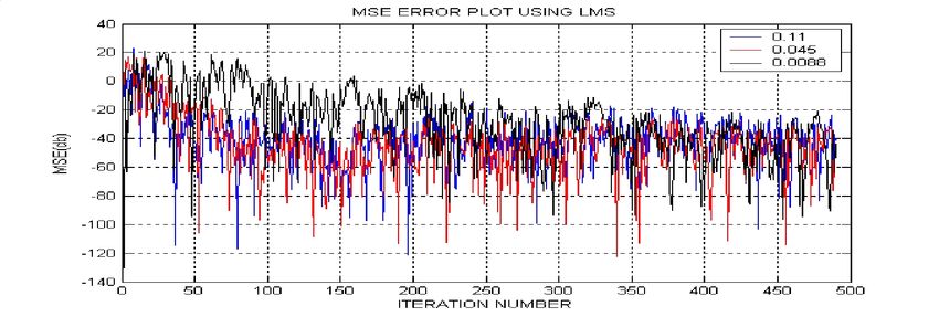
To see the performance of EVSSLMS three different population size (i) 10 (ii) 20 (iii)50, taken for
same input signal as in case(1) and outcome has shown in fig3.it is clear from result performance
is vary very little with higher population size. Plot of adapted vary step size also shown in fig4.the
requirement of initial higher value and later lower value of step size easily captured by
evolutionary programming.
FIGURE 2: fixed step size performance of LMS with step size equal to 0.11, 0.045 and 0.0088
FIGURE 3: performance of EVSSLMS with different population size 10,20 and 50.
Signal Processing: An International Journal (SPIJ), Volume (6) : Issue (2) : 2012 83Ajjaiah H.B.M, P.V.Hunagund, Manoj Kumar Singh & P.V.Rao
FIGURE 4: Defined step size by EVSSLMS for different population size
6. CONCLUSION
The problem of optimal variable step size integrated with LMS algorithm has solved with the
involvement of evolutionary programming. Presented method is robust and does not require the
statistical characteristics of input signal as in the case of other existing solutions. Very good
convergence and tracking capability can be achieved automatically by presented method.
Performance of proposed VSSLMSEV also checked with different population size and it has
shown that with less population performance is also equally well and in result higher speed of
solution.
Acknowledgement
This research is completed at Manuro Tech Research, Bangalore, India and one of author
wanted to say thanks to the management and staff of Jyothi institute of technology, Bangalore,
India for their support.
7. REFERENCE
[1] Solmaz, C.O.; Oruc, O.; Kayran, A.H.; “ Optimal step-size LMS equalizer algorithm
“.Signal Processing and Communications Applications (SIU), 2011 IEEE . April 2011,
pp.853 - 856
[2] Wee-PengAng Farhang-Boroujeny, B,” A new class of gradient adaptive step size LMS
algorithm” ,Signal Processing, IEEE Transactions on,2001, Volume: 49 Issue: 4 , pp: 805 –
810.
[3] Krstajic, B. Stankovic, L.J. Uskokovic, Z. “an approach to variable step size LMS algorithm”.
:Electronics Letters , Aug 2002 ,Volume: 38 Issue: 16,PP: 927 - 928 .
[4] Saul B. Gelfand, Yongbin Wei, James V. Krogmeier, ,” The Stability of Variable Step-Size
LMS Algorithms” IEEE transactions on signal processing, Vol. 47, NO. 12, December 1999.
[5] R. Kwong and E. W. Johnston, “A variable step size LMS algorithm,” IEEE Trans. Signal
Processing, vol. 40, pp. 1633–1642, July 1992.
[6] V. J. Mathews and Z. Xie, “A stochastic gradient adaptive filter with gradient adaptive step
size,” IEEE Trans. Signal Processing, vol. 41, pp. 2075–2087, June 1993.
[7] Tao Dai; Shahrrava, B.,” Variable step-size NLMS and affine projection algorithms with
variable smoothing factor “Circuits and Systems, 2005. 48th Midwest Symposium on, Aug.
2005, pp: 1530 - 1532 ,Vol. 2.
[8] J. H. Husoy and M. S. E. Abadi “Unified approach to adaptive filters and their performance”
IET Signal Processing, vol. 2 , No. 2 , pp. 97-109, 2008.
Signal Processing: An International Journal (SPIJ), Volume (6) : Issue (2) : 2012 84Ajjaiah H.B.M, P.V.Hunagund, Manoj Kumar Singh & P.V.Rao
[9] H. C . Shin and A. H. Sayed “Mean square performance of a family of affine projection
algorithms” IEEE Trans. Signal Processing, vol. 52, pp. 90-102, 2004.
Signal Processing: An International Journal (SPIJ), Volume (6) : Issue (2) : 2012 85You can also read