Advanced Lattice Sieving on GPUs, with Tensor Cores
←
→
Page content transcription
If your browser does not render page correctly, please read the page content below
Advanced Lattice Sieving on GPUs,
                  with Tensor Cores

           Léo Ducas1 and Marc Stevens1 and Wessel van Woerden1

                        CWI, Amsterdam, The Netherlands

      Abstract. In this work, we study GPU implementations of various
      state-of-the-art sieving algorithms for lattices (Becker-Gama-Joux 2015,
      Becker-Ducas-Gama-Laarhoven 2016, Herold-Kirshanova 2017) inside the
      General Sieve Kernel (G6K, Albrecht et al. 2019). In particular, we ex-
      tensively exploit the recently introduced Tensor Cores – originally de-
      signed for raytracing and machine learning – and demonstrate their fit-
      ness for the cryptanalytic task at hand. We also propose a new dual-hash
      technique for efficient detection of ‘lift-worthy’ pairs to accelerate a key
      ingredient of G6K: finding short lifted vectors.
      We obtain new computational records, reaching dimension 180 for the
      SVP Darmstadt Challenge improving upon the previous record for di-
      mension 155. This computation ran for 51.6 days on a server with 4
      NVIDIA Turing GPUs and 1.5TB of RAM. This corresponds to a gain
      of about two orders of magnitude over previous records both in terms of
      wall-clock time and of energy efficiency.

      Keywords: Lattice Sieving, Shortest Vector, G6K, Cryptanalysis, Chal-
      lenges.

1   Introduction

Lattice reduction is a key tool in cryptanalysis at large, and is of course a central
interest for the cryptanalysis of lattice-based cryptography. With the expected
standardisation of lattice-based cryptosystems, the question of the precise per-
formance of lattice reduction algorithms is becoming a critical one. The crux of
the matter is the cost of solving the Shortest Vector Problem (SVP) with sieving
algorithms. While even in the RAM model numerous questions remain regarding
the precise cost of the fastest algorithms, one may also expect a significant gap
between this model and practice, due to their high-memory requirements.
    Lattice sieving algorithms [AKS01, NV08, MV10] are asymptotically supe-
rior to enumeration techniques [FP85, Kan83, SE94, GNR10], but this has only
recently been shown in practice. Recent progress on sieving, both on its theo-
retical [Laa15, BGJ15, BDGL16, HKL18] and practical performances [FBB+ 14,
Duc18, LM18, ADH+ 19], brought the cross-over point with enumeration as low
as dimension 80. The work of Albrecht et al. at Eurocrypt 2019, named the Gen-
eral Sieve Kernel (G6K), set new TU Darmstadt SVP-records [SG10] on a single
machine up to dimension 155, while before the highest record was at 152 using
a cluster with multiple orders of magnitude more core-hours of computation.
Before scaling up to a cluster of computers, a natural step is to port cryptan-
alytic algorithms to Graphical Processing Units (GPUs); not only are GPUs far
more efficient for certain parallel tasks, but their bandwidth/computation capac-
ity ratio are already more representative of the difficulties to expect when scaling
up beyond a single computational server. This step can therefore already teach
us a great deal about how a cryptanalytic algorithm should scale in practice. The
only GPU implementation of sieving so far [YKYC17] did not make use of ad-
vanced algorithmic techniques (such as the Nearest Neighbour Search techniques,
Progressive Sieving or the Dimensions for Free technique [Laa15,LM18,Duc18]),
and is therefore not very representative of the current state of the art.
An important consideration for assessing practical cryptanalysis is the direc-
tion of computation technologies, and one should in particular note the advent of
Tensor architectures [JYP+ 17], offering extreme performance for low-precision
matrix multiplication. While this development has been mostly motivated by
machine learning applications, the potential application for cryptanalytic algo-
rithms must also be considered. Interestingly, such architectures are now also
available on commodity GPUs (partly motivated by ray-tracing applications),
and therefore accessible even with modest resources.
1.1 Contributions
The main contribution of this work is to show that lattice sieving, including
the more complex and recent algorithmic improvements, can effectively be ac-
celerated by GPUs. In particular, we show that the NVIDIA Tensor cores, only
supporting specific low-precision computations, can be used efficiently for lat-
tice sieving. We exhibit how the most computationally intensive parts of complex
sieving algorithms can be executed in low-precision even in large dimensions.
We show and demonstrate by an implementation that the use of Tensor cores
results in large efficiency gains for cryptanalytic attacks, both in hardware and
energy costs. We present several new computational records, reaching dimen-
sion 180 for the TU Darmstadt SVP challenge record with a single high-end
machine with 4 GPUs and 1.5TB RAM in 51.6 days. Not only did we break
SVP-records significant faster, but also with < 4% of the energy cost compared
to a CPU only attack. For instance, we solved dimension 176 using less time and
with less than 2 times the overall energy cost compared to the previous record
of dimension 155. Furthermore by re-computing data at appropriate points in
our algorithms we reduced the memory usage per vector by 60% compared to
the base G6K implementation with minimal computational overhead.
Our work also includes the first implementation of asymptotically best sieve
(BDGL) from [BDGL16] inside the G6K framework, both for CPU-only (multi-
threaded and AVX2-optimized) and with GPU acceleration. We use this to shed
some light on the practicality of this algorithm. In particular we show that our
CPU-only BDGL-sieve already improves over the previous record-holding sieve
2in dimensions as low as 95, but that this cross-over point lies much higher for
our GPU accelerated sieve due to memory-bottleneck constraints.
One key feature of G6K is to also consider lifts of pairs even if such a
pair is not necessarily reducible, so as to check whether such lifts are short;
the more such pairs are lifted, the more dimensions for free one can hope
for [Duc18, ADH+ 19]. Yet, Babai lifting of a vector has quadratic running time
which makes it too expensive to apply to each pair. We introduce a filter based
on dual vectors that detects whether pairs are worth lifting. With adequate pre-
computation on each vector, filtering a pair for lifting can be made linear-time,
fully parallelizable, and very suitable to implement on GPUs.
Open Source Code. Since the writing of this report, our CPU implementation
of bdgl has been integrated in G6K, with further improvements, and we aim for
long term maintenance.1 The GPU implementations has also been made public,
but with lower expectation of quality, documentation and maintenance.2
Acknowledgments. The authors would like to express their gratitude to Joe
Rowell for his precious feedback and support on parts of our code.
The research of L. Ducas was supported by the European Union’s H2020
Programme under PROMETHEUS project (grant 780701) and the ERC-StG-
ARTICULATE project (no. 947821). W. van Woerden is funded by the ERC-
ADG-ALGSTRONGCRYPTO project (no. 740972). The computational hard-
ware enabling this research was acquired thanks to a Veni Innovational Research
Grant from NWO under project number 639.021.645 and to the Google Security
and Privacy Research Award awarded to M. Stevens.
2 Preliminaries
2.1 Lattices and the Shortest Vector Problem
Notation. Given a matrix B = (b0 , . . . , bd−1 ) ⊂ Rd with linearly independent
Pd
columns, we define the lattice generated by the basis B as L(B) := { i xi bi :
xi ∈ Z}. We denote the volume of the fundamental area B · [0, 1]d by det(L) :=
| det(B)|. Given a basis B we define πi as the projections orthogonal to the span
of (b0 , . . . , bi−1 ) and the Gram-Schmidt orthogonalisation as B∗ = (b∗0 , . . . , b∗d−1 )
where b∗i := πi (bi ). The projected sublattice L[l:r] where 0 ≤ l < r ≤ d is defined
as the lattice with basis B[l:r] := (πl (bl ), . . . , πl (br−1 )). Note that the Gram-
Schmidt orthogonalisation of B[l:r] is induced by B∗ and equals (b∗l , . . . , b∗r−1 );
Qr−1
consequently det(L[l:r] ) = i=l kb∗i k. When working with the projected sub-
lattice L[l:r] and the associated basis B[l:r] we say that we work in the context
[l : r].
1
https://github.com/fplll/g6k/pull/61
2
https://github.com/WvanWoerden/G6K-GPU-Tensor
3The Shortest Vector Problem. The computationally hard problem on which
lattice-based cryptography is based relates to the Shortest Vector Problem (SVP),
which given a basis asks for a non-zero lattice vector of minimal length. More
specifically, security depends on approximate versions of SVP, where we only try
to find a non-zero lattice vector at most a factor poly(d) longer than the minimal
length. However, via block reduction techniques like (D)BKZ [SE94, MW16] or
slide reduction [GN08, ALNSD20], the approximate version can be reduced to a
polynomial number of exact SVP instances in a lower dimension.
Definition 1 (Shortest Vector Problem (SVP)) Given a basis B of a lat-
tice L, find a non-zero lattice vector v ∈ L of minimal length λ1 (L) := min kwk.
06=w∈L
For the purpose of cryptanalysis, SVP instances are typically assumed to be
random, in the sense that they are distributed close to the Haar measure [GM03].
While the exact distribution is irrelevant, it is assumed for analysis that these
instances follow the Gaussian Heuristic for ‘nice’ volumes K; which is widely
verified to be true for lattices following the Haar measure.
Heuristic 1 (The Gaussian Heuristic (GH)) Let K ⊂ Rd be a measurable
body, then the number |K ∩ L| of lattice points in K is approximately equal to
Vol(K)/ det(L).
Note that the number of lattice points the Gaussian Heuristic indicates is exactly
the expected number of lattice points in a random translation of K. When
applying the Gaussian Heuristic to a d-dimensional ball of volume det(L) we
obtain that the minimal length λ1 (L) is approximately
p the radius of this ball,
which asymptotically means that λ1 (L) ≈ d/(2πe) · det(L)1/d . For a lattice
L ⊂ Rd we denote this radius by gh(L), and to shorten notation we denote
gh(l : r) := gh(L[l:r] ). In practice for random lattices the minimal length deviates
at most 5% from the predicted value starting around dimension 50, and even
less in larger dimensions [GNR10, Che13]. Note that a ball of radius δ · gh(L)
contains an exponential number of δ d lattice vectors not much longer than the
minimal length. We say that a list of lattice vectors saturates a volume K if
it contains some significant ratio (say 50%) of the lattice vectors in L ∩ K as
predicted by the Gaussian Heuristic.
Lifting and dimensions for free. We discuss how to change context without
increasing the length of vectors too much. Extending the context to the right
(from [l : r] to [l : r + k]) is merely following the inclusion L[l:r] ⊂ L[l:r+k] .
Extending the context on the left is more involved. To lift a vector v from
L[l:r] to L[l−k:r] for 0 ≤ k ≤ l we have to undo the projections away from
b∗l−k , . . . , b∗l−1 . Such a lift is not unique, e.g., if w ∈ L[l−k:r] projects to v, then
so would the infinite number of lattice vectors w − c with c ∈ L[l−k:l] , and our
goal is to find a rather short one.
4w−c
t−c v = πl (w)
0 l−k l r d
Note that we can orthogonally decompose any lift as w − c = (t − c) + v
with t ∈ span(L[l−k:l] ), c ∈ L[l−k:l] and v ∈ L[l:r] . So each lift has squared
2 2
length kt − ck + kvk and to minimize this we need to find a lattice vector
c ∈ L[l−k:l] that lies close to t. Note that even if we find a closest lattice point the
2
added squared length kt − ck is lower bounded by dist2 (t, L[l−k:l] ). Instances for
which this distance is very small are better known as δ-BDD (Bounded Distance
Decoding) instances, where δ indicates the maximum distance of the target to
the lattice.
Finding a close lattice point is at least as hard as finding a short vector,
so for optimal lifts one would need the dimension k to stay small. E.g., for a
1-dimensional lattice the problem is equivalent to integer rounding. A famous
polynomial time algorithm to find a somewhat close lattice point is Babai’s
nearest plane algorithm: lift in 1-dimensional steps [l : r] → [l − 1 : r] →
· · · → [l − k : r], greedily finding the closest lattice point in the 1-dimensional
lattices b∗l−1 Z, . . . , b∗l−k Z. Babai’s nearest plane algorithm finds a lattice point at
Pl−1 2
squared distance at most 14 i=l−k kb∗i k , and always returns the closest lattice
point for δ-BDD instances with δ ≤ 12 minl−k≤idimensions for free technique explained before it makes sense to stop when the
database saturates a ball with some saturation radius R, i.e., when the database
contains a significant ratio of the short lattice vectors of length at most R. A
simple sieving algorithm is summarized in Algorithm 1.
Provably solving SVP with lattice sieving leads to many technical problems
like showing that we can actually find enough short combinations and in partic-
ular that they are new, i.e., they are not present in our database yet; unfortu-
nately side-stepping these technicalities leads to high time and memory complex-
ities [AKS01, MV10, PS09]. In contrast there are also sieving algorithms based
mainly on the Gaussian and similar heuristics and these do fall in the practical
regime. The first and simplest of these practical sieving algorithms by Nguyen
and Vidick uses a database of N = (4/3)d/2+o(d) = 20.2075d+o(d) vectors and runs
in time N 2+o(1) = 20.415d+o(d) by repeatedly checking all pairs v±w [NV08]. The
database size of (4/3)d/2+o(d) is the minimal number of vectors that is needed
in order to keep
p finding enough shorter pairs, and eventually saturate the ball
of radius of 4/3 · gh(L). In a line of works [Laa15, BGJ15, BL16, BDGL16] the
time complexity was gradually improved to 20.292d+o(d) by nearest neighbour
searching techniques to find close pairs more efficiently. Instead of checking all
pairs they first apply some bucketing strategy in which close vectors are more
likely to fall into the same bucket. By only considering the somewhat-close pairs
inside each bucket, the total number of checked pairs can be decreased. In order
to lower the memory requirement of 20.2075d+o(d) one can also look at triplets of
vectors in addition to pairs. This leads to a time-memory trade-off; lowering the
memory cost while increasing the computational cost. The current best triple
sieve with minimal memory 20.1887d+o(d) takes time 20.3588d+o(d) [HKL18].
2.2 The General Sieve Kernel
The General Sieve Kernel (G6K) [ADH+ 19] is a lattice reduction framework
based on sieving algorithms that is designed to be ‘stateful’ instead of treating
sieving as a black-box SVP oracle. This encompasses recent algorithmic progress
like progressive sieving and dimensions for free. Besides an abstract state ma-
chine that allows to easily describe many reduction strategies, it also includes an
Algorithm 1: Lattice sieving algorithm.
Input : A basis B of a lattice L, list size N and a saturation radius R.
Output: A list L of short vectors saturating the ball of radius R.
1 Sample a list L ⊂ L of size N .
2 while L does not saturate the ball of radius R do
3 for every pair v, w ∈ L do
4 if v − w ∈/ L and kv − wk < maxu∈L kuk then
5 Replace a longest element of L by v − w.
6 return L
6open-source implementation that broke several new TU Darmstadt SVP Chal-
lenges [SG10] up to dimension 155. This implementation is multi-threaded and
low-level optimized and includes many of the implementation tricks from the
lattice sieving literature and some more. In this section we recall the state and
instructions of G6K.
State. Naturally, the state includes a lattice basis B ∈ Zd×d and its correspond-
ing Gram-Schmidt basis B̃. The current state keeps track of a sieving context
[l : r] and a lifting context [κ : r]. In the remainder of this work the sieving di-
mension will be denoted by n := r −l. There is a database L containing N lattice
vectors from the sieving context. To conclude G6K also keeps track of good in-
sertion candidates iκ , . . . , il for the corresponding positions in the current lattice
basis.
Instructions. In order to move between several contexts there are several in-
structions like Extend Right, Shrink Left and Extend Left. To avoid
invalidating the database the vectors are lifted to the new context as explained
in Section 2.1, keeping the lifted vectors somewhat short. The Insertion in-
struction inserts one of the insertion candidates back into the basis B, replacing
another basis vector, and the Gram-Schmidt basis B̃ is updated correspond-
ingly. By some carefully chosen transformations and by moving to the slightly
smaller sieving context [l + 1 : r] we can recycle most of the database after an
insertion. We can also Shrink the database by throwing away the longest vec-
tors or Grow it by sampling new (long) vectors. The Sieve instruction reduces
vectors in the database until saturation of a ball of a given radius. G6K also
allows for well-chosen vectors that are encountered during sieving to be lifted
from the sieving context [l : r] to hopefully short vectors in the lifting context
[κ : r], and storing the best insertion candidates. The Sieve instruction is agnos-
tic about the sieving algorithm used, which allows to relatively easily implement
and then compare sieving algorithms with each other, while letting G6K take
care of global strategies.
Global Strategies. The implementation of G6K consists of a high level Python
layer and a low-level C++ layer. The earlier mentioned instructions can be called
and parametrized from the Python layer, while the core implementation con-
sists of highly optimized C++ code. This allows one to quickly experiment with
different global strategies. An important global strategy is known as the pump
up: start in a small context of say [d − 40 : d] and alternate the Extend Left,
Grow and Sieve instructions until the context reaches a certain dimension
(passed as a parameter). Note that the sieve in each dimension already starts
with a database consisting of many relatively short vectors, thus taking signif-
icantly less iterations to complete. This technique is also known as progressive
sieving [Duc18, LM18] and gives a significant practical speed-up. A full pump
consists of a pump up followed by a pump down: repeat the Insertion instruc-
tion to improve the basis while making the context smaller again, and optionally
combine this with the Sieve instruction to find better insertion candidates. To
7solve SVP-instances among other things G6K combines such pumps in a work-
out, which is a sequence of longer and longer pumps, until a short enough vector
is found in the full context by lifting. Each pump improves the quality of the
basis, which as a result lowers the expected length increase from lifting, making
consequent pumps faster and simultaneously improving the probability to find
a short vector in the full context.
G6K Sieve implementations. The current open-source implementation of
G6K contains multiple sieving algorithms that implement the Sieve instruc-
tion. There are single-threaded implementations of the Nguyen–Vidick sieve (nv)
[NV08] and Gauss sieve (gauss) [MV10], mostly for testing purposes. Further-
more G6K includes a fully multi-threaded and low-level optimized version of the
Becker–Gama–Joux (BGJ) sieve with a single bucketing layer (bgj1) [BGJ15].
The filtering techniques from bgj1 were also extended and used in a triple sieve
implementation (triple) [BLS16, HK17]. This implementation considers both
pairs and triples and its behaviour automatically adjusts based on the database
size, allowing for a continuous time-memory trade-off between the (pair) sieve
bgj1 and a full triple sieve with minimal memory. Note that the asymptotically
best sieve algorithm, which we will refer to as BDGL, has been implemented
before [BDGL16, MLB17], but not inside of G6K.
Data representation. Given that lattice sieving uses an exponential number
of vectors, it is of practical importance how much data is stored per vector
in the database. G6K stores for each lattice vector v = Bx ∈ Rn the (16-
bit integer) coordinates x ∈ Zn as well as the (32-bit floating-point) Gram-
Schmidt representation y = (hv, b∗i i/ kb∗i k)i ∈ Rn normalized by the Gaussian
Heuristic of the current sieving context. The latter representation is used to
quickly compute inner products between any two lattice vectors in the database.
On top of that other preprocessed information is stored for each vector, like the
corresponding lift target t in span(L[κ:l] ), the squared length, a 256-bit SimHash
(see [Cha02, FBB+ 14, Duc18]) and a 64-bit hash as identifier. In order to sort
the database on length, without having to move the entries around, there is also
a lightweight database that only stores for each vector the length, a SimHash
and the corresponding database index. A hash table keeps track of all hash
identifiers, which are derived from the x-coordinates, in order to quickly check
for duplicates. All of this quickly adds up to a total of ≈ 210 bytes per vector in
a sieving dimension of n = 128.
3 Architecture
3.1 GPU Device Architecture
In this section we give a short summary of the NVIDIA Turing GPU architecture
on which our implementations and experiments are based. During the write-up
of this paper a new generation named Ampere was launched, doubling many of
the performance metrics mentioned here.
8GPU SM 1 GPU Peak Performance: GPU SM 68
max. 1024 threads Clock: 1545MHz max. 1024 threads
FP32: 13.4 TFLOPS
64 CC 8 TC FP16: 26.9 TFLOPS 64 CC 8 TC
FP16-TU: 107.6 TFLOPS
Registers Registers
64K × 32-bit 64K × 32-bit
99GB/s 99GB/s
L1 Shared L1 Shared
32KiB/ 64KiB/ 32KiB/ 64KiB/
System RAM
64KiB 32KiB 64KiB 32KiB
1.5TiB
(≈ 1270GB/s)
GPU L2 Cache
5.5MiB
616GB/s
GPU RAM 16GB/s
System CPU(s)
11GiB
Fig. 1. Device architecture of the NVIDIA RTX 2080 Ti used in this work.
CUDA cores and memory. A NVIDIA GPU can have up to thousands of
so-called CUDA cores organized into several execution units called Streaming
Multiprocessors (SM ). These SM use their many CUDA cores (e.g. 64) to service
many more resident threads (e.g. 1024), in order to hide latencies of computation
and memory operations. Threads are bundled per 32 in a warp, that follow the
single-instruction multiple-data paradigm.
The execution of a GPU program, also called a kernel, consists out of multiple
blocks, each consisting of some warps. Each individual block is executed on any
available single SM. The GPU RAM, also called global memory, can be accessed
by all cores. Global memory operations always pass through a GPU-wide L2
cache. In addition, each SM benefits from a individual L1 cache and offers an
addressable shared memory that can only be used by threads in that block.
In this work we focus on the NVIDIA RTX2080 Ti that we used, whose
architecture is depicted in Figure 1. While a high-end CPU with many cores
can reach a performance in the order of a few tera floating point operations per
second (TFLOPS), the RTX2080 Ti can achieve 13 TFLOPS for 32-bit floating
point operations on its regular CUDA cores.
To implement GPU kernel functions for a NVIDIA GPU one can use CUDA
[NBGS08, NVF20] which is an extension of the C/C++ and FORTRAN program-
ming languages. A kernel is executed by a specified number of threads grouped
into blocks, all with the same code and input parameters. During execution each
thread learns that it is thread t inside block b and one needs to use this informa-
tion to distribute the work. For example when loading data from global memory
we can let thread t read the t-th integer at an offset computed from b, because
the requested memory inside each block is contiguous such a memory request
can be executed very efficiently; such memory request are known as coalescing
reads or writes and they are extremely important to obtain an efficient kernel.
9Tensor cores. Driven by the machine learning domain there have been tremen-
dous efforts in the past few years to speed up low-precision matrix multiplica-
tions. This lead to the so-called Tensor cores, that are now standard in high-end
NVIDIA GPUs. Tensor cores are optimized for 4 × 4 matrix multiplication and
also allow a trade-off between performance and precision. In particular we are
interested in the 16-bit floating point format fp16 with a 5-bit exponent and a
10-bit mantissa, for which the tensor cores obtain an 8× speed-up over regular
32-bit operations on CUDA cores.
Efficiency. For cryptanalytic purposes it is not only important how many op-
erations are needed to solve a problem instance, but also how cost effective these
operations can be executed in hardware. The massively-parallel design of GPUs
with many relatively simple cores results in large efficiency gains per FLOP com-
pared to CPU designs with a few rather complex cores; both in initial hardware
cost as in power efficiency.
As anecdotal evidence we compare the acquisition cost, energy usage and
theoretical peak performance of the CPU and GPU in the new server we used
for our experiments: the Intel Xeon Gold 6248 launched in 2019 and the NVIDIA
RTX2080 Ti launched in 2018 respectively. The CPU has a price of about e2500
and a TDP of 150 Watt, while the GPU is priced at about e1000 and has a
TDP of 260 Watt. For 32-bit floating point operations the peak performance is
given by 3.2 TFLOPS3 and 13.45 TFLOPS for the CPU and GPU respectively,
making the GPU a factor 2.4 better per Watt and 10.5 better per Euro spend on
acquisition. For general 16-bit floating point operations these number double for
the GPU, while the CPU obtains no extra speed-up (one actually has to convert
the data back to 32-bit). When considering the specialized Tensor cores with
16-bit precision the GPU has a theoretical peak performance of 107.6 TFLOPS,
improving by a factor 19.4 per Watt and a factor 84 per Euro spend on acquisition
compared to the CPU.
3.2 Sieve Design
The great efficiency of the GPU is only of use if the state-of-the-art algorithms
are compatible with the massively-parallel architecture and the specific low-
precision operations of the Tensor cores. To show this we extended the lattice
sieving implementation of G6K. We will focus our main discussion on the sieving
part, as the other G6K instructions are asymptotically irrelevant and relatively
straightforward to accelerate on a GPU (which we also did).
All of our CPU multi-threaded and GPU-powered sieve implementations fol-
low a similar design (cf. Fig. 2) consisting out of three sequential phases: bucket-
ing, reducing and result insertion. We call the execution of this triplet an iteration
and these iterations are repeated until the desired saturation is achieved. Note
that our sieves are not ‘queued’ sieves such as the Gauss-Sieve of [MV10] and the
3
With 64 FLOP per core per cycle using two AVX-512 FMA units and a maximal clock
frequency of 2500MHz when using AVX-512 on all 20 cores.
10Database
Bucketing Reducing Insertion
Loop until target saturation achieved
Fig. 2. High level diagram of the implemented Sieving process.
previous record setting triple_sieve; this relaxation aligns with the batched
nature of GPU processing and allows to implement an asymptotically optimal
BDGL-like sieve [BDGL16], without major memory overhead.
Bucketing. During the bucketing phase, the database is subdivided in several
buckets B1 , . . . , Bm ⊂ L, each containing relatively close vectors. We do not
necessarily bucket our full database, as some vectors might be too large to be
interesting for the reduction phase in the first few iterations. For each bucket we
collect the database indices of the included vectors. For the sieves we consider,
these buckets can geometrically be interpreted as spherical caps or cones with
for each bucket Bk an explicit or implicit bucket center ck ∈ Rn indicating its
direction. For each included vector v ∈ Bk , we also store the inner product hck , vi
with the bucket center, which is obtained freely from the bucketing process.
Note that a vector may be included in several buckets, something which we
tightly control by the multi-bucket parameter, whose value we will denote by
M . The optimal amount of buckets m and the expected number of vectors in a
bucket differs for each of our bucketing implementations. In Section 4, we further
exhibit our different bucketing implementations and compare their performance
and quality.
Reducing. During the reduction phase, we try to find all close pairs of lattice
vectors inside each bucket, i.e., at distance at most some length bound `. Using
negation, we orient the vectors inside a bucket into the direction of the bucket
center based on the earlier computed inner product hck , vi i. In case the bucketing
center ck is itself a lattice vector (as can be the case for BGJ-like sieves, but not
for BDGL), it is also interesting to check if ck − vi − vj is a short lattice vector,
leading to a triple reduction [HK17].
For each bucket Bk , we compute all pairwise inner products hvi , vj i for
vi , vj ∈ Bk . Together with the already computed lengths kvi k , kvj k , kck k and
inner products hck , vi i, hck , bj i we can then efficiently decide if vi − vj or
ck − vi − vj is short. Note that we compute the length of both the pair and
the triple essentially from a single inner product computation. We return the
indices of pairs and triplets that result in a vector of length at most the length
bound `, together with the length of the new vector. In Section 5 we further dis-
cuss the reduction phase, and in Appendix B and exhibit implementation details
of our reduction kernel on the GPU using low-precision Tensor cores.
11The number of inner products we have to compute per bucket grows quadrat-
icly in the bucket size |Bk |, while the number of buckets only decreases linearly
in the bucket size. Therefore, one would in principle want many buckets that
are rather small and of high quality, improving the probability that a checked
pair actually gives a reduction. For a fixed bucketing algorithm more buckets
generally increase the cost of the bucketing phase, while decreasing the cost of
the reduction phase due to smaller bucket sizes. We try to balance the cost of
these phases to obtain optimal performance.
Next to finding short vectors in the sieving context we also want to find pairs
that lift to short vectors in the larger lifting context. Unfortunately it is too
costly to just lift all pairs as this has a cost of at least Θ((l − κ)2 ) per pair.
In Section 6 we introduce a filter based on dual vectors that can be computed
efficiently for each pair given a bit of pre-computed data per vector. The few
pairs that survive this filter are more likely to lift to a short vector and we only
lift those pairs.
Result insertion. After the sieving part we have a list of tuples with indices and
the corresponding length of the new vector they represent. The hash identifier
of the new vector can efficiently be recomputed by linearity of the hash function
and we check for duplicates in our current database. For all non-duplicate vectors
we then compute their x-representation. After all new entries are created they
are inserted back in the database, replacing entries of greater length.
3.3 Data storage and movement
Recall from Section 2.2 that G6K stores quite some data per vector such as
the coefficients x in terms of the basis, a Gram-Schmidt representation y, the
lift target t, a SimHash, and more. Theoretically we could remove all data ex-
cept the x-representation and compute all other information on-the-fly. How-
ever, as most of this other information has a cost of Θ(n2 ) to compute from
the x-representation this would mean a significant computational overhead, for
example increasing the cost of an inner product from Θ(n) to Θ(n2 ). Also given
the limited amount of performance a CPU has compared to a GPU we certainly
want to minimize the amount of such overhead for the CPU. By recomputing
at some well chosen points on the GPU, our accelerated sieves minimize this
overhead, while only storing the x-representation, length and a hash identifier
per vector, leading to an approximately 60% reduction in storage compared to
the base G6K implementation. As a result we can sieve in significantly larger
dimensions with the same amount of system RAM.
While GPUs have an enormous amount of computational power, the mem-
ory bandwidth between the database in system RAM and the GPU’s RAM is
severely limited. These are so imbalanced that one can only reach theoretical
peak performance with Tensor cores if every byte that is transferred to the GPU
is used in at least 213 computations. A direct result is that reducing in small
buckets is (up to some threshold) bandwidth limited. Growing the bucket size
in this regime would not increase the wall-clock time of the reduction phase,
12while at the same time considering more pairs. So larger buckets are preferred,
in our hardware for a single active GPU the threshold seems to be around a
bucket size of 214 , matching the 213 computations per byte ratio. Because in
our hardware each pair of GPUs share their connection to the CPU, halving the
bandwidth for each, the threshold grows to around 215 when using all GPUs
simultaneously. The added benefit of large buckets is that the conversion from
the x-representation to the y-representation, which can be done directly on the
GPU, is negligible compared to computing the many pairwise inner products. To
further limit the movement of data we only return indices instead of a full vector;
2
if we find a short pair vi −vj on the GPU we only return i, j and kvi − vj k . The
new x-representation and hash identifier can efficiently (in O(n)) be computed
on the CPU directly from the database.
4 Bucketing
The difference between different lattice sieve algorithms mainly lies in their
bucketing method. These methods differ in their time complexity and their
performance in catching close pairs. In this section we exhibit a Tensor-GPU
accelerated bucketing implementation triple_gpu similar to bgj1 and triple
inspired by [BGJ15, HK17], and two optimized implementations of the asymp-
totically best known bucketing algorithm [BDGL16], one for CPU making use
of AVX2 (bdgl) and one for GPU (bdgl_gpu). After this we show the practical
performance difference between these bucketing methods.
4.1 BGJ-like bucketing (triple gpu)
The bucketing method used in bgj1 and triple is based on spherical caps di-
rected by explicit bucket centers that are also lattice points. To start the buck-
eting phase we first choose some bucket centers b1 , . . . , bm from the database;
preferably the directions of these vectors are somewhat uniformly distributed
over the sphere. Then each vector v ∈ L in our database is associated to bucket
Bkv with
bk0
kv = arg max ,v .
1≤k0 ≤m kbk0 k
We relax this condition somewhat by the multi bucket parameter M , to associate
a vector to the best M buckets. In this we differ from the original versions of bgj1
and triple [BGJ15, HK17, ADH+ 19] in that they use a fixed filtering threshold
on the angle |hbk / kbk k , v/ kvki|. As a result our buckets do not exactly match
spherical caps, but they should still resemble them; in particular such a change
does not affect the asymptotic analysis. We chose for this alternation as this fixes
the amount of buckets per vector, which reduced some communication overhead
in our highly parallel GPU implementations.
In each iteration the new bucket centers are chosen, normalized and stored
once on each GPU. Then we stream our whole database v1 , . . . , vN through the
13GPUs and try to return for each vector the indices of the M closest normalized
bucket vectors and their corresponding inner products hvi , bk i. For efficiency rea-
sons the bucket centers are distributed over 16 threads and each thread stores
only the best encountered bucket for each vector. Then we return the buckets
from the best M ≤ 16 threads, which are not necessarily the best M buckets
overall. The main computational part of computing the pairwise inner prod-
ucts is similar to the Tensor-GPU implementation for reducing, and we refer to
Appendix B for further implementation details.
The cost of bucketing is O(N · n) per bucket. Assuming that the buckets are
of similar size |Bk | ≈ M · N/m the cost to reduce is O( Mm·N · n) per bucket.
√
To balance these costs for an optimal runtime one should choose m ∼ M · N
buckets per iteration. For the regular 2-sieve strategy with an asymptotic mem-
ory usage of N = (4/3)n/2+o(n) = 20.208n+o(n) this leads to a total complexity of
20.349n+o(n) using as little as 20.037n+o(n) iterations. Note that in low dimensions
we might prefer a lower number of buckets to achieve the minimum required
bucket size to reach peak efficiency during the reduction phase.
4.2 BDGL-like bucketing (bdgl and bdgl gpu)
The asymptotically optimal bucketing method from [BDGL16] is similar to bgj1
as in that it is based on spherical caps. The difference is that in contrast to
bgj1 the bucket centers are not arbitrary but structured, allowing to find the
best bucket without having to compute the inner product with each individual
bucket center.
Following [BDGL16], such a bucketing strategy would look as follows. First
we split the dimension n into k smaller blocks (say, k = 2, 3 or 4 in practice)
of similar dimensions n1 , . . . , nk that sum up to n. In order to randomize this
splitting over different iterations one first applies a random orthonormal trans-
formation Q to each input vector. Then the set C of bucket centers is constructed
as a direct product of random local bucket centers, i.e., C = C1 × ±C2 · · · × ±Ck
with Cb ⊂ Rnb . Note that for a vector v we only have to pick the closest local
bucket centers
Q to find the closest global bucket center,Pimplicitly considering
m = 2k−1 b |Cb | bucket centers at the cost of only b |Cb | ≈ O(m
1/k
) in-
ner products. By sorting the local inner products we can also efficiently find
all bucket centers within a certain angle or say the closest M bucket centers.
With similar reasons as for triple_gpu we always return the closest M bucket
centers for each vector instead of a fixed threshold based on the angle. While for
a fixed number of buckets m we can expect some performance loss compared to
bgj1 as the bucket centers are not perfectly random, this does not influence the
asymptotics.4
To optimize the parameters we again balance the cost of bucketing and re-
ducing. Note that for k = 1 we essentially obtain bgj1 with buckets of size
O(N 1/2 ) and a time complexity of 20.349n+o(n) . For k = 2 or k = 3 the buckets
become smaller of size O(N 1/3 ) and O(N 1/4 ) respectively and of higher quality,
4
The analysis of [BDGL16, Theorem 5.1] shows this is up to a sub-exponential loss.
14leading to a time complexity of 20.3294n+o(n) and 20.3198n+o(n) respectively. By
letting k slowly grow, e.g., k = O(log(n)) there will only be a sub-exponential
2o(n) number of vectors in each bucket, leading to the best known time complex-
ity of 20.292n+o(n) . Note however that a lot of sub-exponential factors might be
hidden inside this o(n), and thus for practical dimensions a rather small value
of k might give best results.
We will take several liberties with the above strategy to address practical
efficiency consideration and fine-tune the algorithm. For example, for a pure
CPU implementation we may prefer to make the average bucket size somewhat
larger than the ≈ N 1/(k+1) vectors that the theory prescribes; this will improve
cache re-use when searching for reducible pairs inside buckets. In our GPU im-
plementation, we make this average bucket size even larger, to prevent memory
bottlenecks in the reduction phase.
Furthermore, we optimize the construction of the local bucket centers c ∈ Ci
to allow for a fast computation of the local inner products hc, vi. While [BDGL16]
choose the local bucket centers Ci uniformly at random, we apply some extra
structure to compute each inner product with a vector v in time O(log(ni ))
instead of O(ni ). The main idea is to use the (Fast) Hadamard Transform H
on say 32 ≤ ni coefficients of v. Note that this computes the inner product
between v and 32 orthogonal ternary vectors, which implicitly form the bucket
centers, using only 32 log2 (32) additions or subtractions. To obtain more than
32 different buckets we permute and negate coefficients of v in a pseudo-random
way before applying H again. This strategy can be heavily optimized both for
CPU using the vectorized AVX2 instruction set (bdgl) and for GPU by using
special warp-wide instructions (bdgl gpu). In particular this allows a CPU core
to compute an inner product every 1.3 to 1.6 cycles for 17 ≤ ni ≤ 128. For
further implementation details we refer to Appendix A.
Since the writing of this report, our CPU implementation of bdgl has been
integrated in G6K, with further improvements.5 As it may be of independant
interest, the AVX2 bucketer is also provided as a standalone program.6
4.3 Quality Comparison
In this section we compare the practical bucketing quality of the BGJ- and
BDGL-like bucketing methods we implemented. More specifically, we consider
triple_gpu, 1-bdgl_gpu and 2-bdgl_gpu where the latter two are instances of
bdgl_gpu with k = 1 and k = 2 blocks respectively. Their quality is compared to
the idealized theoretical performance of bgj1 with uniformly distributed bucket
centers.7 For triple_gpu, we follow the Gaussian Heuristic and sample bucket
centers whose directions are uniformly distributed. As a result the quality dif-
ference between triple_gpu and the idealized version highlights the quality loss
5
https://github.com/fplll/g6k/pull/61
6
https://github.com/lducas/AVX2-BDGL-bucketer
7
Volumes of caps and wedges for predicting the idealized behavior where ex-
tracted from [AGPS19], and more specifically https://github.com/jschanck/
eprint-2019-1161/blob/main/probabilities.py.
15resulting from our implementation decisions. Recall that compared to bgj1 the
main difference is that for every vector we return the M closest bucket centers
instead of using a fixed threshold for each bucket. Also these are not exactly the
M closest bucket centers, as we first distribute the buckets over 16 threads and
only store a single close bucket per thread. For our bdgl_gpu implementation
the buckets are distributed over 32 threads and we add to this that the bucket
centers are not random but somewhat structured by the Hadamard construction.
To compare the geometric quality of bucketing implementations, we mea-
sure how uniform vectors are distributed over the buckets and how many close
pairs end up in at least one common bucket. The first measure is important
as the reduction cost does not depend on the square of the average bucket size
1
Pm 2
mP k=1 |Bk | , which is fixed, but on the average of the squared bucket size
1 m 2
m k=1 |Bk | , which is only minimal if the vectors are equally distributed over
the buckets. For all our experiments we observed at most an overhead of 0.2%
compared to perfectly equal bucket sizes and thus we will further ignore this part
of the quality assessment. To measure the second part efficiently we sample 220
close unit pairs (x, y) ∈ S n × S n uniformly at random such that hx, yi = ± 12 .
Then we count the number of pairs that have at least 1 bucket in common, possi-
bly over multiple iterations. We run these experiments with parameters that are
representative for practical runs. In particular we consider (sieving) dimensions
up to n = 144 and a database size of N = 3.2 · 20.2075n to compute the number
of buckets given the desired average bucket size and the multi-bucket parameter
M . Note that we specifically consider the geometric quality of these bucketing
implementations for equivalent parameters and not the cost of the bucketing
itself.
To compare the bucketing quality between the different methods and the
idealized case we first consider the experimental results in graphs a. and b.
of Figure 3. Note that the bucketing methods triple_gpu and 1-bdgl_gpu
obtain extremely similar results overall, showing that the structured Hadamard
construction is competitive with fully random bucket centers. We see a slight
degradation of 5% to 20% for triple_gpu with respect to the idealized case as a
result of not using a fixed threshold. We do however see this gap decreasing when
M grows to 4 or 8, indicating that these two methods of assigning the buckets
become more similar for a larger multi-bucket parameter. At M = 16 we see a
sudden degradation for triple_gpu which exactly coincides with the fact that
the buckets are distributed over 16 threads and we only store the closest bucket
per thread. The quality loss of 2-bdgl_gpu seems to be between 15% and 36%
in the relevant dimensions, which is quite significant but reasonable given a loss
potentially as large as sub-exponential [BDGL16, Theorem 5.1].
Now we focus our attention on graph c. of Figure 3 to consider the influ-
ence of the average bucket size on the quality. We observe that increasing the
average bucket size reduces the bucketing quality; many small buckets have a
better quality than a few large ones. This is unsurprising as the asymptotically
optimal BDGL sieve aims for high quality buckets of small size. Although our
k-bdgl_gpu bucketing method has no problem with efficiently generating many
16a. (n = 128, |Bk | ≈ 214 ) b. (M = 4, |Bk | ≈ 214 )
1
Found Pairs (relative)
0.5
N/A
0
1 2 4 8 16 96 112 128 144
Multi Bucket (M ) Dimension (n)
c. (n = 128, M = 4)
0.6
Found Pairs (ratio)
Iterations = 216 / Bucket Size
0.4
0.2
0
210 211 212 213 214 215 216
Average Bucket Size (|Bk |)
Idealized triple gpu 1-bdgl gpu 2-bdgl gpu
Fig. 3. Bucketing Quality Comparison. We sampled 220 pairs v, w of unit vectors such
that |hv, wi| = 0.5 and we measured how many fell into at least 1 common bucket.
The number of buckets is computed based on the desired average bucket size |Bk |, the
multi-bucket parameter M , and a representative database size of N = 3.2 · 20.2075n .
The found pairs in a. and b. are normalized w.r.t. idealized theoretical performance
of bgj1 (perfectly random spherical caps). For c. the number of applied iterations is
varied such that the total reduction cost is fixed.
small buckets, the reduction phase cannot efficiently process small buckets due to
memory bottlenecks. This is the main trade-off of (our implementation of) GPU
acceleration, requiring a bucket size of 215 versus e.g. 210 leads to a potential
loss factor of 7 to 8 as shown by this graph. For triple_gpu this gives no major
problems as for the relevant dimensions n ≥ 130 the optimal bucket sizes are
large enough. However 2-bdgl_gpu should become faster than bgj1 exactly by
considering many smaller buckets of size N 1/3 instead of N 1/2 , and a minimum
bucket size of 215 shifts the practical cross-over point above dimension 130, and
potentially much higher.
5 Reducing with Tensor cores
Together with bucketing, the most computationally intensive part of sieving
algorithms is that of finding reducing pairs or triples inside a bucket. We con-
17sider a bucket of s vectors v1 , . . . , vs ∈ Rn with bucket center c. Only the x-
representations are send to the GPU and there they are converted to the 16-bit
Gram-Schmidt representations y1 , . . . , ys and yc that are necessary to quickly
2
compute inner products. Together with the pre-computed squared lengths ky1 k ,
2
. . . , kys k and inner products hyc , y1 i, . . . , hyc , ys i, the goal is to find all pairs
yi −yj or triples yc −yi −yj of length at most some bound `. A simple derivation
shows that this is the case if and only if
2 2
kyi k + kyj k − `2
for pairs: hyi , yj i ≥ , or
2
2 2 2
kyc k + kyi k + kyj k − `2 − 2hyc , yi i − 2hc, yj i
for triples: hyi , yj i ≤ − .
2
And thus we need to compute all pairwise inner products hyi , yj i. If we consider
the matrix Y := [y1 , . . . , ys ] ∈ Rn×s then computing all pairwise inner products
is essentially the same as computing one half of the matrix product Yt Y.
Many decades have been spend optimizing (parallel) matrix multiplication for
CPUs, and this has also been a prime optimization target for GPUs. As a result
we now have heavily parallelized and low-level optimized BLAS (Basic Linear
Algebra Subprograms) libraries for matrix multiplication (among other things).
For NVIDIA GPUs close to optimal performance can often be obtained using
the proprietary cuBLAS library, or the open-source, but slightly less optimal
CUTLASS library. Nevertheless the BLAS functionality is not perfectly adapted
to our goal. Computing and storing the matrix Yt Y would require multiple
gigabytes of space. Streaming the result Yt Y to global memory takes more time
than the computation itself. Indeed computing Yt Y using cuBLAS does not
exceed 47 TFLOPS for n ≤ 160, and this will be even lower when also filtering
the results.
For high performance, in our implementation we combined the matrix mul-
tiplication with result filtering. We made sure to only return the few indices of
pairs that give an actual reduction to global memory; filtering the results locally
while the computed inner products are still in registers. Nevertheless the data-
movement design, e.g. how we efficiently stream the vectors yi into the registers
of the SMs, is heavily inspired by CUTLASS and cuBLAS. To maximize memory
read throughput, we had to go around the dedicated CUDA tensor API and re-
verse engineer the internal representation to obtain double the read throughput.
Further implementation details are discussed in Appendix B.
Efficiency. To measure the efficiency of our Tensor-accelerated GPU kernel we
did two experiments: the first experiment runs only the kernel with all (con-
verted) data already present in global memory on the GPU, while the second
experiment emulates the practical efficiency by including all overhead. This over-
head consists of obtaining the vectors from the database, sending them to the
GPU, converting them to the appropriate representation, running the reduction
kernel, recomputing the length of the resulting close pairs, and retrieving the
results from the GPU. Each experiment processed a total of 228 vectors of di-
mension 160 in a pipelined manner on a single NVIDIA RTX 2080 Ti GPU and
1870 Excluding overhead
Including overhead
60
16-bit TFLOPS 50
40
30
20
10
0
210 211 212 213 214 215 216
Bucket Size
Fig. 4. Efficiency of the reduction GPU kernel for different bucket sizes on a RTX 2080
Ti, only counting the 2n FLOPS per inner product. The overhead includes obtaining
the vectors from the database, sending them to the GPU, conversions, recomputing
length at higher precision, and retrieving the results from the GPU in a pipelined
manner.
with a representative number of 10 CPU threads. We only counted the 2n 16-bit
floating point operations per inner product and not any of the operations nec-
essary to transfer data or to filter and process the results. The theoretical limit
for this GPU when only using Tensor cores and continuously running at boost
clock speeds is 107 TFLOPS, something which is unrealistic in practice.
The results of these experiments are displayed in Figure 4. We see that the
kernel itself reaches around 65 TFLOPS starting at a bucket size of at least
212 . When including the overhead we see that the performance is significantly
limited below a bucket size of 213 which can fully be explained by CPU-GPU
memory-bottlenecks. For bucket sizes of at least 214 we see that the overhead
becomes reasonably small. We observed that this threshold moves to 215 when
using multiple GPUs, because in our hardware the CPU-GPU bandwidth is
shared per pair of GPUs.
Precision. The main drawback of the high performance of the tensor cores is
that the operations are at low precision. Because the runtime of sieving algo-
rithms is dominated by computing pairwise inner products to find reductions or
for bucketing (in case of triple_gpu) we focus our attention on this part. Other
operations like converting between representations are computationally insignif-
icant and can easily be executed by regular CUDA cores at higher precisions.
As the GPU is used as a filter to find (extremely) likely candidates for reduc-
tion, we can tolerate some relative error, say up to 2−7 in the computed inner
product, at the loss of more false positives or missed candidates. Furthermore it
19√
2−8 Max (2−13.613 · n)
√
99th percentile (2−14.313 · n)
−16.005
√
2−9 Average (2 · n)
Computation Error 2−10
2−11
2−12
2−13
2−14
16 32 64 128 256 512 1024 2048
Dimension (n)
Fig. 5. Computation error |S − Ŝ| observed in dimension n over 16384 sampled pairs
of unit vectors y, y0 that satisfy S := hy, y0 i ≈ 0.5.
is acceptable for our purposes if say 1% of the close vectors are missed because
of even larger errors. In Appendix C we show under a reasonable randomized
error model that problems due to precision are insignificant up to dimensions as
large as n = 2048. This is also confirmed by practical experiments as shown in
Figure 5.
6 Filtering Lifts with Dual Hash
Let us recall the principle of the ‘dimensions for free’ trick [Duc18]; by lifting
many short vectors in the sieving context [l : r] we can recover a short(est)
vector in some larger context [l − k : r] for k > 0. The sieving implementation
G6K [ADH+ 19] puts extra emphasis on this by lifting any short pair it encounters
while reducing a bucket, even when this vector is not short enough to be added
to the database. Note that G6K first filters on the length in the sieving context
because lifting has a significant cost of O(n · k + k 2 ) per pair. The O(n · k) part
to compute the corresponding target ti − tj ∈ Rk in the context [l − k : l] can
be amortized to O(k) over all pairs by pre-computing t1 , . . . , ts , leaving a cost
of O(k 2 ) for the Babai nearest plane algorithm.
We went for a stronger filter with an emphasis on the extra length added by
the lifting. Most short vectors will lift to rather large vectors, as by the Gaussian
Heuristic we can expect an extra length of gh(l − k : l)
gh(l − k : r). For the
few lifts that we are actually interested in we expect an extra length of only
δ · gh(l − k : l), for some 0 < δ < 1 (say δ ∈ [0.1, 0.5] in practice). This means
that we need to catch those pairs ti − tj that lie exceptionally close to the lattice
[l − k : l], also known as BDD instances.
20More abstractly we need a filter that quickly checks if pairs are (exception-
ally) close over the torus Rk /L. Constructing such a filter directly for this
rather complex torus and our practical parameters seems to require at least
quadratic time like Babai’s nearest plane algorithm. Instead we introduce a
dual hash to move the problem to the much simpler but possibly higher di-
mensional torus Rh /Zh . More specifically, we will use inner products with short
dual vectors to build a BDD distinguisher in the spirit of the so-called dual at-
tack on LWE given in [MR09] (the general idea can be traced back at least
to [AR05]). This is however done in a different regime, where the shortest
dual vectors are very easy to find (given the small dimension of the consid-
ered lattice); we will also carefully select a subset of those dual vectors to op-
timize the fidelity of our filter. Recall that the dual of a lattice L is defined as
L∗ := {w ∈ span(L) : hw, vi ∈ Z for all v ∈ L}.
Definition 1 (Dual hash). For a lattice L ⊂ Rk , h ≥ k and a full (row-rank)
matrix D ∈ Rh×k with rows in the dual L∗ , we define the dual hash
HD : Rk /L → Rh /Zh ,
t 7→ Dt.
The dual hash relates distances in Rk /L to those in Rh /Zh .
Lemma 2. Let L ⊂ Rk be a lattice with some dual hash HD . Then for any
t ∈ Rk we have
dist(HD (t), Zh ) ≤ σ1 (D) · dist(t, L),
where σ1 (D) denotes the largest singular value of D.
Proof. Let x ∈ L such that kx − tk = dist(t, L). By definition we have Dx ∈ Zh
and thus HD (t−x) ≡ HD (t). We conclude by noting that dist(HD (t−x), Zh ) ≤
kD(t − x)k ≤ σ1 (D) kt − xk.
So if a target t lies very close to the lattice then HD (t) lies very close to Zh . We
can use this to define a filter that passes through BDD instances.
Definition 3 (Filter). Let L ⊂ Rk be a lattice with some dual hash HD . For
a hash bound H we define the filter function
1, if dist(HD (t), Zh ) ≤ H,
FD,H : t 7→
0, else.
Note that computing the filter has a cost of O(h · k) for computing Dt for
D ∈ Rh×k followed by a cost of O(h) for computing dist(Dt, Zh ) using simple
coordinate-wise rounding. Given that h ≥ k, computing the filter is certainly
not cheaper than ordinary lifting, which is the opposite of our goal. However
this changes when applying the filter to all pairs ti − tj with 1 ≤ i < j ≤ h.
We can pre-compute Dt1 , . . . , Dts once, which gives a negligible overhead for
large buckets, and then compute D(ti − tj ) by linearity, lowering the total cost
to O(h) per pair.
216.1 Dual Hash Analysis
We further analyse the dual hash filter and try to understand the correlation
between the distance dist(t, L) and the dual hash HD (t). In fact we consider
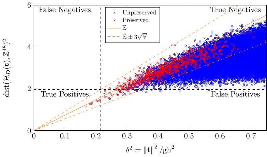
two regimes, the preserved and unpreserved regime. Consider a target t ∈ Rk
and let x be a closest vector in L to t. We will say that we are in the preserved
regime whenever D(t − x) ∈ [− 21 , 12 ]h (i.e., Dx remains a closest vector of Dt
among Zh ), in which case it holds that kD(t − x)k2 = dist(HD (t), Zh ). In the
general case, we only have the inequality kD(t − x)k2 ≥ dist(HD (t), Zh ). For
the relevant parameters, the BDD instances we are interested in will fall almost
surely in the preserved regime, while most of the instances we wish to discard
quickly will fall in the unpreserved regime.
Preserved Regime. We have that kD(t − x)k2 = dist(HD (t), Zh ), and there-
fore Lemma 2 can be complemented with a lower bound as follows:
σk (D) · dist(t, L) ≤ dist(HD (t), Zh ) ≤ σ1 (D) · dist(t, L).
Setting a conservative hash bound based on the above upper bound leads to
false positives of distance at most σ1 (D)/σk (D) further away than the targeted
BDD distance. This is a worst-case view, however, and we are more interested in
the average behavior. We will assume without loss of generality that x = 0, such
that dist(t, L) = ktk. To analyse what properties play a role in this correlation
we assume that t is spherically distributed for some fixed length ktk. Suppose
that Dt D has eigenvalues σ12 , . . . , σk2 with corresponding normalized (orthogo-
Pk
nal) eigenvectors v1 , . . . , vk . We can equivalently assume that t = i=1 ti vi
with (t1 , . . . , tk )/ ktk uniformly distributed over the sphere. Computing the ex-
pectation and variation we see
" k # k k
2 1
2
X X X
2 2 2 2
E[kDtk ] = E ti · σi = σi · E[ti ] = ktk · σ2
i=1 i=1
k i=1 i
k k
!2
4
h
2
i ktk 1 X 1 X
Var kDtk = · σ4 − σ2 .
(k/2 + 1) k i=1 i k i=1 i
So instead ofqthe worst case bounds from Lemma 2, dist(HD (t), Zh ) is more or
Pk
less close to k1 i=1 σi2 · ktk.
Unpreserved Regime. In this regime dist(HD (t), Zh ) is not really a useful
metric, as there will seemingly be no relation with kD(t − x)k2 . Note that we can
expect this regime to mostly contain targets that lie rather far from the lattice,
i.e., these are targets we want to not pass our filter. Therefore it is interesting
to analyse how many (false) positives we can expect from this regime.
Inspired by practical observations, we analyse these positives from the heuris-
tic assumption in this regime that every Dt is just uniformly distributed over
22You can also read