Ambiguous Information and Dilation: An Experiment* - Denis Shishkin
←
→
Page content transcription
If your browser does not render page correctly, please read the page content below
Ambiguous Information and Dilation: An Experiment*
Denis Shishkin† ® Pietro Ortoleva‡

This version: June 9, 2021
Latest version available here

Abstract
With standard models of updating under ambiguity, new information may increase the amount of relevant
ambiguity: the set of priors may ‘dilate.’ We test experimentally one sharp case: agents bet on a risky urn
and get information that is truthful or not based on the draw from an Ellsberg urn. With common models,
the set of priors should dilate, and the value of bets decrease for ambiguity-averse individuals, increase if
ambiguity-seeking. Instead, we find that the value of bets does not change for ambiguity-averse agents; it
increases substantially for ambiguity-seeking ones. We also test bets on ambiguous urns and find sizable
reactions to ambiguous information.

Keywords: Updating, Ambiguous Information, Ambiguity Aversion, Ellsberg Paradox, Maxmin Expected Utility.

JEL: C91, D81, D90.

* We   thank Marina Agranov, Simone Cerreia-Vioglio, Mark Dean, David Dillenberger, Adam Dominiak, Yoram Halevy, Faruk
Gul, Yucheng Liang, Fabio Maccheroni, Massimo Marinacci, Stephen Morris, Wolfgang Pesendorfer, Leeat Yariv, and Sevgi
Yuksel for useful comments and suggestions. We are grateful to Rui Tang for excellent research assistance. Ortoleva
gratefully acknowledges the financial support of NSF Grant SES-1763326. The ® symbol indicates that the authors’ names
are in random order.
† Department of Economics, University of California San Diego. Email: dshishkin@ucsd.edu.
‡ Department of Economics and SPIA, Princeton University. Email: pietro.ortoleva@princeton.edu.
1    Introduction

An extensive theoretical and experimental literature has studied modeling and implications of
ambiguity—when payoffs depend on states of the world for which there is no objective proba-
bility distribution. A fundamental aspect, especially for applications, is how ambiguity interacts
with updating. However, the theoretical literature in this area seems further from a consensus, and
experimental analysis is much less extensive.
    We study experimentally one aspect of ambiguity and updating: how agents react to information
of ambiguous reliability. Agents make bets and receive messages that can be truthful or misleading
depending on the draw from an Ellsberg urn. We study this for three reasons.
    First, this tests a key implication of standard models of updating under ambiguity: that information
may increase relevant ambiguity and make agents worse off —the so-called ‘dilation’ of sets of priors.
For example, with widespread updating rules for MaxMin Expected Utility, the set of relevant priors
may become larger (dilate) after information. This makes ambiguity-averse agents strictly worse off
after information; they should be willing to pay to avoid it. Appealing or not, this is an implication of
widespread models. To our knowledge, it has not been tested. Our experiment with information of
ambiguous reliability allows us to test a very sharp case, in which dilation should occur after any
message—‘all news is bad news’ (Gul and Pesendorfer, 2018).
    Second, the dilation feature of updating that we test is central to many applications to game
theory and mechanism design. In fact, the very type of ambiguous information we study in our
experiment is used in applications: below, we discuss papers that include ambiguity to mechanism
design and Bayesian persuasion and in which, in the motivating examples of both, the ambiguity lies
in having messages that are either truthful or not, exactly like in our experiment.
    Third, more in general, our experiment contributes to the growing interest in ambiguous in-
formation, focusing on the case of ambiguity on the reliability of messages. While ambiguity in
informativeness may be commonplace in real life, it is studied only by very few recent papers, discussed
below.

Experiment.     Subjects first evaluate bets on the color of a ball drawn from an urn. In some cases,
they receive a message about the winning color; this message is truthful or misleading depending on
the draw from a (separate) 2-color Ellsberg bag of chips. After subjects acknowledge the message,
we measure how the value of bets changes. We also measure the (positive or negative) value of this
information. In some questions, the payoff-relevant draw is made from a risky, 50/50 urn; thus, all
ambiguity is in the message. In other questions, draws are made from an ambiguous urn. We also
measure subjects’ ambiguity-aversion.

Relation to Theories.    Standard models of updating under ambiguity make clear predictions. Con-
sider the MaxMin Expected Utility model (MMEU) of Gilboa and Schmeidler (1989). Two updating

                                                   1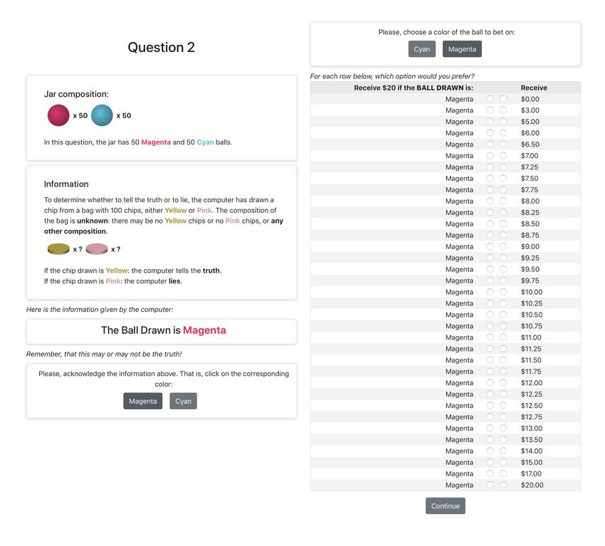
rules are widespread: Full-Bayesian (FB), where the posterior set includes updates of all priors; and
Maximum-Likelihood (ML), where the updated set includes only priors that satisfy a maximum-
likelihood criterion. When the payoff-relevant state is risky, the relevant set of priors without
information is a singleton. But after ambiguous information, as in our experiment, with FB or ML the
relevant set of priors dilates and is no longer a singleton: because of the ambiguity in information,
bets on the risky urn become ambiguous. Ambiguity-averse individuals should then decrease the value
of bets after information, and even pay to avoid it. (The opposite is true for ambiguity-seeking.) Note
that these predictions hold for any message, meaning that all news is bad news.
    One may well consider unappealing some of these predictions—especially that information must
make ambiguity-averse individuals strictly worse off. They are, however, central implications of these
theories and crucial to applications. We test them.
    We also show that these predictions hold beyond MMEU: they also apply to Bayesian updating
of (symmetric) Smooth Ambiguity model (Klibanoff, Marinacci, and Mukerji, 2005, 2009). As this
model is very different from MMEU, this points to how pervasive this implication is.

Results.   When the payoff-relevant state is risky, ambiguity-averse or neutral subjects typically
do not change the value of bets after information. The median change is zero, and the majority
has exactly zero change. For ambiguity-averse subjects, there is also no robust relation between
ambiguity-aversion and the size of change (or the probability it is non-zero). They also typically
give zero value to information. All these findings contrast to the theoretical predictions of negative
reaction to information and negative value of information.
    Ambiguity-seeking subjects instead typically increase their valuation after information, and the
change in value is strongly related to their ambiguity affinity, in line with the theoretical prediction.
Yet, many still value the information close to zero.
    When the payoff-relevant state is ambiguous, ambiguity-averse subjects slightly increase valua-
tions, ambiguity-seeking subjects decrease them. Theories make no prediction for this case.

Implications. We conclude the paper by discussing implications. We found that ambiguity-averse
agents do not react negatively to our type of ambiguous information, contradicting the dilation
property of widespread models of updating under ambiguity. Because this property is crucial in
applications, we discuss alternative rules.
    First, subjects may be using FB or ML, but complement it by strategically choosing if to process the
information. While with Subjective Expected Utility information is always weakly valuable—ignoring
it gives no benefit—this is no longer the case under ambiguity. Thus, subjects may decide to ignore
information when harmful. To our knowledge, the only existing model with this feature is Dynamically
Consistent Updating (Hanany and Klibanoff, 2007, 2009), where agents form an ex-ante optimal
plan contingent on information and use an updating rule such that they want to implement it. This
rule, however, violates consequentialism, in the sense that unrealized parts of the decision problem

                                                   2
may influence beliefs.
Alternatively, subjects may follow Proxy Updating (Gul and Pesendorfer, 2018) or Conditional
Maximum Likelihood (Tang, 2020), which satisfy consequentialism but restricts dilation. Proxy
Updating is designed precisely to rule out instances of ‘all news is bad news’. While the exact model
cannot be applied to our setup—it is defined for totally monotone capacities, which is not the case
here—our results are strongly supportive of this approach. Conditional Maximum Likelihood is
defined for MMEU, always results in a unique posterior, and is compatible with our main finding that
ambiguity-averse agents do not change their valuation of bets after information.
Literature. A theoretical literature discusses updating rules under ambiguity (Gilboa and Marinacci,
2013, Sec. 5), while an experimental one tested dynamic consistency and consequentialism (Cohen,
Gilboa, Jaffray, and Schmeidler, 2000; Dominiak, Duersch, and Lefort, 2012; Bleichrodt, Eichberger,
Grant, Kelsey, and Li, 2018; Esponda and Vespa, 2019), how sampling from ambiguous sources affects
ambiguity preferences (Ert and Trautmann, 2014), learning from sequences of observations (Moreno
and Rosokha, 2016), in groups (De Filippis, Guarino, Jehiel, and Kitagawa, 2016), or from stock
prices (Baillon, Bleichrodt, Keskin, L’Haridon, and Li, 2017).
Three very recent papers study ambiguous information: Epstein and Halevy (2019), Liang (2019),
and Kellner, Le Quement, and Riener (2019).1 A common difference with our work is that they
do not study the dilation property, our primary focus. Building on Epstein and Schneider (2007,
2008), Epstein and Halevy (2019) defines and characterizes attitudes to ‘signal ambiguity,’ the
ambiguity on the informativeness of a signal, and tests it experimentally.2 Focusing on a setup with
ambiguity, they find that signal ambiguity significantly increases deviations from Bayesian updating.
While related to our work in the interest on ambiguous signals, in Epstein and Halevy (2019) the
payoff-relevant state is ambiguous and signals are always informative, but the agent does not know
how much; instead, in our experiment the payoff-relevant state can be risky and the ambiguity is on
whether the signal is informative or misleading. The papers are thus complementary: our design is
less extensive on ambiguous information but allows us to test the dilation property and a form of
ambiguous information used in the applied literature.
A contemporaneous paper by Liang (2019) studies updating with risky state under simple and
uncertain (ambiguous and compound) signals; and ambiguous and compound state under simple
signals. It compares updating under different types of signals that correspond to the same average
simple signal and finds that subjects under-react to uncertain information, which is more pronounced
for good news rather than bad news. Also contemporaneous, Kellner, Le Quement, and Riener (2019)
studies messages with ambiguous reliability, but asymmetric and with three messages, one of which
1 Moreover, Vinogradov and Makhlouf (2020) augment the Ellsberg experiment with vague statements about an
ambiguous payoff-relevant state, which may be perceived as ambiguous signals. Kops and Pasichnichenko (2020) find a
negative value of risky signals with an ambiguous payoff-relevant state.
2 We learned about Epstein and Halevy (2019) before finalizing our design. We thank Yoram Halevy for useful discussions.
3is informative. They find a relation between reactions and ambiguity attitude; and a similar reaction
to ambiguous and compound-risk signals. Their design does not allow tests of dilation.
Lastly, as noted above, the ambiguous information we study is used in applications of models of
ambiguity to strategic environments. Bose and Renou (2014) study mechanism design where the
allocation stage is preceded by an ambiguous mediated communication stage; Beauchêne, Li, and Li
(2019) study Bayesian persuasion with an ambiguity-averse receiver and a sender who can commit
to ambiguous signals. Both papers assume FB and their results are linked to its dilation property.
Pahlke (2019) and Cheng (2020) study ambiguous persuasion under alternative updating rules that
account for dynamic consistency and dilation.
2 Theories of Updating and Ambiguous Information
Consider a set of prizes X = R and a state space S = Ω × M , where Ω = { R, B } are the payoff-relevant
states (colors of the ball), and M = {r, b} the messages.
Assume preferences are represented by MMEU: given strictly increasing, continuous utility
u : X → R and set of priors Π ⊆ ∆(S), agents evaluate act f : S → X by min Eπ [u ◦ f ] if ambiguity-
π ∈Π
averse; replacing min with max if ambiguity-seeking.
Given Π , let Π Ω denote the set of marginals over Ω and identify any π̂ ∈ Π Ω with π̂( R) ∈ [0, 1].
In line with our experiment, assume that, for all priors, the likelihood that a message is truthful
or not is independent of the payoff-relevant state, i.e., π(r | R) = π(b | B). Moreover, assume that Π
contains the uninformative prior π̄ (i.e., π̄(r | R) = π̄(b | R) = 0.5) and, if |Π| , 1, it does so in its
relative interior. We call coherent any closed set of priors that satisfies these restrictions.
Updating Rules. For any event D ⊆ S, let Π D denotes the set of beliefs after information D. The
following two updating rules are most common.
Full Bayesian (FB) updating (Wasserman and Kadane, 1990; Jaffray, 1992; Pires, 2002; Ghirardato,
Maccheroni, and Marinacci, 2008), the most common in applications, is defined by
FB
Π D B {π(·| D) : π ∈ Π}.
Maximum Likelihood (ML) (Dempster, 1967; Shafer, 1976; Gilboa and Schmeidler, 1993) is
defined by
ML
Π D B {π(·| D) : π ∈ argmax π 0( D)}.
π ∈Π
0
Under FB, individuals update all priors following Bayes’ rule. Under ML, they retain (and update)
only the priors with the highest likelihood of the realized event.
4Variables of Interest. Suppose the individual is ambiguity-averse and consider a bet that pays a
baseline of x and adds y if a color chosen by the individual realizes. Its certainty equivalent is
cm ( x, y ) B u −1
max min π(ω)u( x + y ) + (1 − π(ω))u( x ) ,
ω ∈ { R, B } π ∈Πm
Ω
where m ∈ {, r, b} denotes either the message received or no information (letting Π B Π ).
Our first variable of interest is the Information Premium: the difference between certainty
equivalents of such bets before and after a message,
Pm B cm ( x, y ) − c ( x, y ).
Our second variable of interest is the Value of Information V : the amount V that makes the
individual indifferent between no information and receiving a message while modifying payoffs by V ,
u(c ( x, y )) B min Eπ [u(cm ( x − V, y ))] .
π ∈Π
For ambiguity-seeking individuals, define variables analogously, replacing min with max.
Risky payoff-state. Suppose that the payoff-relevant state is risky.
Proposition 1. Consider a MMEU agent with coherent set of priors Π such that the payoff-state is risky
( |Π Ω | = 1) and symmetric (π( R) = 0.5, ∀π ∈ Π ).3 Then with FB and ML for any m ∈ M :
1. if ambiguity-averse and |Π| > 1: Pm < 0, V < 0;
2. if ambiguity-seeking and |Π| > 1: Pm > 0, V > 0;
3. if ambiguity-neutral (i.e., |Π| = 1): Pm = V = 0.
The proposition shows that ambiguity-averse individuals must have negative Information Premia
Pm for any message m; and a negative Value of Information V . Both are positive if ambiguity-seeking.
For intuition, suppose Π = {π1, π2, π3 } with π1 (r | R) = 0.8 (messages point in the right direction),
π2 (r | R) = 0.5 (messages uninformative), and π3 (r | R) = 0.2 (messages misleading). Before informa-
tion, the set of marginals over Ω was a singleton—we have a risky state. But after information this
set becomes full-dimensional: FB ΠrΩ = FB ΠbΩ = [0.2, 0.8] ⊃ {0.5} = Π Ω . The multiplicity of priors
about the truthfulness of the message generates multiple beliefs about payoff-relevant states. The set
of posteriors not only includes the original prior, but does so in its interior. Importantly, this holds
for any message. Seidenfeld and Wasserman (1993) call this property of FB dilation. Proposition 1
shows that dilation occurs whenever |Π| > 1.
3 Symmetry of the payoff-relevant marginal is assumed only for ease of exposition. Without it, predictions with FB are
the same; with ML, it remains true that both P and V are not zero unless there is ambiguity-neutrality.
5With FB, because the set of priors dilates, ambiguity-averse individuals have strictly lower certainty
equivalents; because this holds for any message, the value of information is negative. The opposite
holds for ambiguity-seeking.
With ML, individuals focus only on priors that maximize the likelihood of the message. When
π(R) = 0.5 for all π ∈ Π , however, the likelihood of both messages is 0.5: thus, all priors in Π are
considered and ML coincides with FB.
Ambiguous payoff-state. Consider now ambiguous payoff-relevant states.
Proposition 2. Consider a MMEU individual with coherent set of priors Π . Then with FB and ML:
1. If |Π| > 1, then both Pm and V can be zero, negative, or positive under both ambiguity-aversion
and seeking;
2. If |Π| = 1, then Pm = V = 0, ∀m ∈ M .
When the payoff-relevant state is ambiguous there are no predictions. Results depend on the
set of priors across Ω and informativeness: Appendix B.1 contains examples showing dilation and
contraction.
Beyond MMEU? Similar results hold beyond MMEU. Consider another popular model, the Smooth
Model (Klibanoff, Marinacci, and Mukerji, 2005). Preferences are represented by
U ( f ) = Eµ [φ(Eπ [u ◦ f ])]
where the continuous, strictly increasing φ : R → R captures ambiguity attitude and µ ∈ ∆(∆(S))
denotes the prior over priors. Following the literature, assume that the individual updates µ following
Bayes’ rule.4 Define Pm and V analogously using this model.
Proposition 3. Consider an individual whose preferences follow the Smooth Model with µ symmetric5
and such that supp(µ) is coherent. If the payoff-state is risky ( | supp(µ)Ω | = 1), then for any m ∈ M :
1. if ambiguity-averse (strictly concave φ): Pm < 0, V < 0;
2. if ambiguity-seeking (strictly convexφ): Pm > 0, V > 0;
3. if ambiguity-neutral (affine φ): Pm = V = 0.
4 Identicalresults also hold if individuals simply update the priors in the support (and not the prior over priors).
5µ is symmetric if for any Q ⊂ ∆(S), µ(Q ) = µ(0.5 − Q ), where 0.5 − Q B {π 0 ∈ ∆(S) : ∃π ∈ Q, ∀s ∈ S, π 0 (s) =
0.5 − π(s)}.
63 Experiment
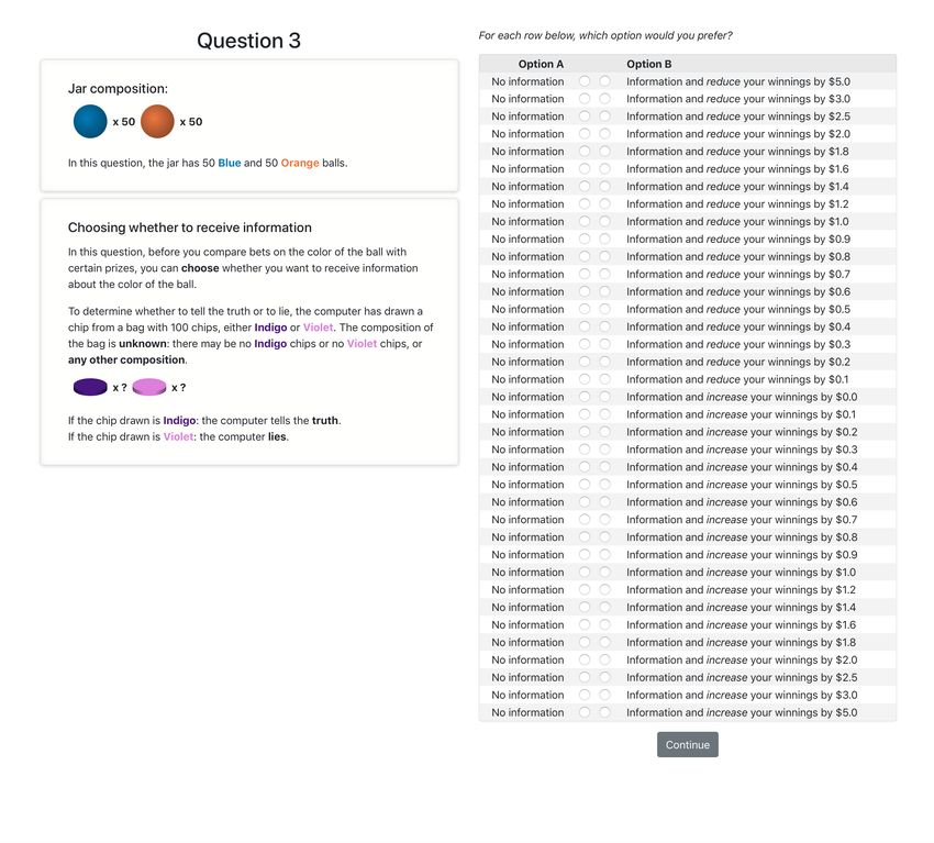
3.1 Design
The experiment includes two parts for a total of 6 questions. In each, subjects were asked to compare
fixed amounts of money with a bet on their chosen color drawn from an urn. With two exceptions
mentioned below, all bets paid $20 if the ball was of the chosen color, zero otherwise; subjects were
asked to compare each bet with a list of amounts of money increasing from $0 to $20, in a Multiple
Price List (MPL). To simplify the task, subjects had to click only once in each list, indicating the point
where to switch from the bet to the amount of money.6
Different questions involved urns of two types. Risky urns had a known composition: 100 balls,
50 of each color. Ambiguous urns had 100 balls of two colors with unknown composition.
Questions were of three kinds. For each, subjects answered one question where the payoff-relevant
urn was risky, and one in which it was ambiguous.
1. Basic Questions. Q1 and Q4 asked subjects to pick a color to bet on and then the certainty
equivalent of a $20 bet using the MPL procedure. In Q1, the urn was risky. In Q4, it was
ambiguous. Comparing the answers, we obtain a measure of ambiguity-aversion.
2. Information Questions. Q2 and Q5 measured the certainty equivalent of a bet, but after infor-
mation. At the beginning of the question, the computer drew a ball from the payoff-relevant
urn—determining the color that pays the bet—and a chip from a bag with 100 chips of 2 colors
and unknown composition. The computer then displayed a message for the subject indicating
the color of the ball drawn from the urn. Whether this message was truthful or misleading,
however, depended on the chip drawn: if the chip was of one color, the computer told the truth;
otherwise, it reported the opposite. In these questions, subjects are first shown the urn, then
shown how the message is determined, then given the message. They then had to acknowledge
it, clicking on the corresponding color. With the message remaining on screen, they had to
pick a color to bet on, and evaluate the bet using an MPL. In Q2, the payoff-relevant urn was
risky; in Q5, it was ambiguous.
3. Information-Value Questions. Q3 and Q6 were similar to the questions above, but also measured
the value of information. In these questions, subjects first faced a MPL in which they chose
between no information and information plus an increase or decrease of their potential winning
for the question (from a base of $20), ranging from −$5 to $5. After their choice, the computer
randomly picked a line from this MPL and implemented their selection: if in that line the
6 By monotonicity, subjects should prefer bets against low amounts and ‘switch’ as the amount grows. The software
(oTree; Chen, Schonger, and Wickens, 2016) asked to indicate the point where to switch. Subjects were also allowed
to indicate no switch (always bet or always money). This procedure simplified choice but forced monotonicity. Subjects
received extensive instruction and training.
7Table 1: Questions
Payoff Urn Info
Q1 Risky No
Part I Q2 Risky Yes
Q3 Risky Evaluate
Q4 Ambiguous No
Part II Q5 Ambiguous Yes
Q6 Ambiguous Evaluate
subject chose no information, they proceeded with the evaluation of the bet without it; if they
chose the information and a change in payoffs, they received both before evaluating the bet. In
Q3, the underlying urn was risky; in Q6, it was ambiguous.
All questions used different urns and different colors, reducing the possibility of hedging across
questions. This was clearly explained. Similarly, the bags that determined the information were all
different and involved different colors. For symmetry, all colors for urns and bags were randomly
selected.7
Order and Incentives. The 6 questions were grouped into two parts. Part I included the 3 questions
involving bets on risky urns, in the following order: Q1, the evaluation of a bet on a risky urn; Q2,
the evaluation of a bet on a risky urn after information; Q3, the evaluation of a bet on a risky urn
after deciding whether to receive or not the information. Part II was identical, but with ambiguous
urns. Questions are summarized in Table 1. There were two possible orders: in Order A, Part I then
Part II; the opposite in Order B.
Subjects received a participation fee of $10 and a completion fee of $15. One of the 6 questions
was randomly selected for payment, and one of the lines of the MPL with the comparison between
bets and amounts of money were randomly selected. Subjects received their choice for that line.8
3.2 Predictions and Construction of Variables
We now map the theoretical predictions from Section 2 to our experiment. From the MPLs comparing
bets and amounts of money, we approximate the certainty equivalent of each bet. From the MPLs
7 Colors were selected randomly for each subject and each question from the same set, except that for each subject we
avoided repetitions and pairings of similar colors.
8 Paying one randomly selected question is incentive compatible under Expected Utility but not beyond; no general
incentive compatible mechanism exists (Karni and Safra, 1987; Azrieli, Chambers, and Healy, 2018). Some studies indicate
this may not be a concern (Beattie and Loomes, 1997; Cubitt, Starmer, and Sugden, 1998; Hey and Lee, 2005; Kurata,
Izawa, and Okamura, 2009), others suggest caution (Freeman, Halevy, and Kneeland, 2019).
8comparing information vs. no information (in Q3 and Q6), we approximate the value of information.
Because in our experiment choices involve different urns, we have to make two assumptions.
First, that Π before information is the same in questions of the same type. This is justified by the
use of identical urns with colors randomly drawn. Second, that subjects’ ambiguity attitude is the
same across questions and with respect to information- and payoff-relevant states, as we have done
implicitly in Section 2. In particular, we assume that if Π Ω is not a singleton when the payoff-state is
ambiguous, then the set of beliefs about the truthfulness of messages is also not a singleton.
We identify ambiguity attitudes comparing the answer to Q1 (risky urn, no info) and Q4 (ambigu-
ous urn, no info): a higher/equal/lower certainty equivalent in Q1 than in Q4 indicates ambiguity-
aversion/neutrality/seeking. The Ambiguity Premium is the difference between the value in Q1 and
the value in Q4.
The Information Premium P is defined as the value in Q2 (Q5) minus the value in Q1 (Q4) for
risky (ambiguous) payoff-state. The Value of Information V is elicited directly in the first part of Q3
(Q6) for risky (ambiguous) payoff-state.9
Applying the results from Section 2, the predictions for risky payoff-states are that both the
Information Premium and the Value of Information should be negative/zero/positive for individuals
that are ambiguity-averse/neutral/seeking. For ambiguous payoff-states the only prediction is that
both measures should be zero for ambiguity-neutral.
Constructing Variables. Because MPLs have finite grids, our value elicitation is approximate. Fol-
lowing standard practice, we define the value as the mid-point between the grid points where the
switch occurred.10 However, the true certainty equivalent may be anywhere in that range and the
approximation may matter in computing if variables are equal, smaller, or bigger than zero. We take
the following conservative approach. Recall that the Information Premium is the difference between
two certainty equivalents, each obtained via a MPL. When computing whether it is above, at, or below
zero, we report it in two ways: first, using the procedure above, and denote results by > 0, = 0, < 0.
Second, we report the percentage of answers that are are compatible with zero value, and denote
them by ≈ 0.11
For the Value of Information, the grid is $0.1 around 0, and 0 is an option on the grid. By our
mid-point construction, no subject can have a value of 0: even if they give 0 value to information,
they must have either 0.05 and −0.05. In calculations, we use these numbers; in reporting > 0, = 0,
9 Note that the second part of Q3 (Q6) was equivalent to Q1 (Q4) or to Q2 (Q5) depending on whether a subject
received information. In such cases, a majority chose consistently.
10 For example, if the individual chose the bet against $10 but the next grid point, say $10.2, against the bet, we set the
certainty equivalent at $10.1.
11 For example, suppose in Q1 the switch is between $10 and $10.2; in Q2, it is one line below, between $10.2 and $10.5.
With our procedure, values are 10.1 for Q1 and 10.35 for Q2, indicating a positive difference. But this behavior is also
compatible with an individual who has zero difference: the true certainty equivalent may be $10.2 in both questions, but
the individual may break indifference in different ways. This behavior is thus marked > 0 but also ≈ 0.
9or < 0, we put 0.05 and −0.05 in = 0 category. Thus, zero values may be overestimated.
Finally, we take a (standard) conservative approach to compute ambiguity attitudes: we classify as
ambiguity-averse or seeking only subjects whose behavior is not compatible with ambiguity-neutrality;
thus, subjects who switch in two adjacent lines in Q1 and Q4 are classified as ambiguity-neutral.12
This implies that we may be overestimating ambiguity-neutral individuals. (As will be clear below,
our main conclusions would not change with different classifications.)
3.3 Results
91 volunteer undergraduate students participated in 4 sessions of approximately 30 minutes run in
the PeXL laboratory in Princeton University in February 2019. Average earnings were $35.2. We
eliminated from our analysis 2 subjects who reported strictly dominated answers in multiple questions.
Including them changes almost nothing (Appendix C.2). Recall that used two different orders. While
this had some effect, our patterns hold throughout with minor differences (Appendix C.1).
The distribution of ambiguity-averse, neutral, seeking is 35 (39.3%), 37 (41.6%), 17 (19.1%).13
Median ambiguity premia are relatively large for both averse ($2.5) and seeking subjects (−$2).
(Table 4 in Appendix C.1 contains all details.)
3.3.1 Risky payoff-state
We begin with the case in which payments depend on a draw from a risky urn. Results appear on
the left of Table 2 and in Figure 1. There, the top panel includes a scatter plot of the Information
Premium and the Ambiguity Premium. Colors represent ambiguity attitude: red for averse, blue for
neutral, green for seeking. On the right is a stacked bar plot depicting the proportions of values that
are > 0, < 0 and = 0. The bottom panel repeats this for the Value of Information.
Considering all subjects, the mean Information Premium P is positive but the median is zero. The
mean Value of Information V is slightly negative, while the median is compatible with zero. To test
the theoretical predictions, however, we have to separate our analysis by ambiguity attitude.
Ambiguity-averse Subjects. For ambiguity-averse subjects, the median Information Premium is
zero: a majority (57%) have a value of exactly zero, 69% has values compatible with zero (denoted
≈ 0). Only for 31% have negative values.
A coherent picture emerges with the Value of Information: it is zero for most ambiguity-averse
subjects. (Recall that −0.05 is compatible with indifference with zero). Of the minority with non-zero
values, the larger group (37%) has negative values.
We can also test the relation between the degree of ambiguity-aversion and the reaction to
information: Are subjects with higher ambiguity premium more likely to have negative, or smaller,
12 Like above, individuals may have the same certainty equivalent but break the indifference in opposite ways.
13 The fraction of ambiguity-averse is lower than general population results (Camerer, Chapaman, Ortoleva, and Snowberg,
2018) but in line with selective universities. Recall that our procedure may overestimate ambiguity-neutral individuals.
10Figure 1: Results, Risky Payoff-Relevant State, Graphically
(a) Information Premium P
15
100
>0
>0
10 80
>0
Information Premium P
P (%, by attitude)
5 60 =0
0 40
=0
=0
−5 20
0
2 80
=0
Value of Information V
V (%, by attitude)
=0
60
0
=0
40
−2Table 2: Results
Risky payoff state Ambiguous payoff state
ambiguity attitude All averse neutral seeking All averse neutral seeking
Information Premium P
theory prediction 0 - 0 -
median 0 0 0 1 0 0 0 −1
mean 0.46 −0.56 0.6 2.2 0.13 0.57 0.08 −0.68
≈0 65% 69% 78% 29% 58% 54% 76% 29%
=0 56% 57% 68% 29% 52% 49% 70% 18%
>0 28% 11% 30% 59% 24% 34% 14% 24%
0 10% 11% 5% 18% 10% 14% 5% 12%A Quantile regression with all subjects finds no relation (t = 0.00, p = 1).
There is also no relation between the Value of Information and the Ambiguity Premium (t =
0.91, p = 0.369).
Ambiguity-seeking Subjects. Patterns are different for ambiguity-seeking subjects: 59%, have
positive Information Premium. Both median and mean are also remarkably high. That is, ambiguity-
seeking subjects substantially increase their valuation after ambiguous information.
The Value of Information, however, remains zero for the majority of them. This suggests that
they do not expect to react positively to messages; but they do once confronted with them. (Dy-
namic inconsistencies are not surprising in this context.) Recall, however, that our procedure may
overestimate how many subjects give zero value to information (Section 3.2).
Figure 1 also suggests a relation between Ambiguity Premium and Information Premium for
ambiguity-seeking subjects. Regressing the two we find a significant, positive relationship (t =
−3.91, p = 0.001). Note, however, that this relation could be spuriously strengthened by our design,
as discussed above. There is no relation with the Value of Information (t = −1.09, p = 0.292).
Ambiguity-neutral Subjects. Ambiguity-neutral subjects exhibit a large majority of zero values
(non-zeros tend to positive and small). About half has zero Value of Information. Interestingly, 43%
give strictly negative values, hinting to non-instrumental role of information.
3.3.2 Ambiguous payoff-state
Results for ambiguous payoff-states appear on the right part of Table 2 and in Figure 2. Clear, but
different patterns emerge. Considering all subjects, the median Information Premium is again zero,
but the mean is slightly positive. The majority still reports zero. Similar results hold for the Value of
Information, albeit with a small, negative mean.
Ambiguity-averse subjects have again a median Information Premium close to zero; a sizable
fraction has Value of Information either zero or compatible with it. But these are smaller fractions
than above and 34% have strictly positive Information Premium.
The opposite pattern holds for ambiguity-seeking subjects: now a majority (59%) has negative
Information Premium. The Value of Information, however, remain predominantly zero in both cases.
Ambiguity-neutral subjects, unsurprisingly, exhibit patterns similar to those found with risky
urns.
Overall, we have a positive relationship between the Information Premium and the Ambiguity
Premium (t = 2.73, p = 0.008), but this does not hold separately for ambiguity-averse (t = 0.95, p =
0.349) or seeking (t = 1.80, p = 0.091) subjects. There is also no relation with the Value of Information
(t = 0.97 overall; t = 1.44 for averse; t = −1.15 for seeking).
13Figure 2: Results, Ambiguous Payoff-Relevant State, Graphically
(a) Information Premium P
10.0
100
>0
7.5
>0
>0
80
5.0
Information Premium P
=0
P (%, by attitude)
2.5
60
0.0 =0
=0
40
−2.5
0
2 80
Value of Information V
V (%, by attitude)
=0
=0
60
0 =0
40
−2
203.4 Comparison with Theory
Common theoretical models predict that with risky state, ambiguity-averse individuals should have
negative Information Premium and Value of Information. Instead, we find that the majority has zero
for both. Only a minority (31%) has negative Information Premium. For ambiguity-seeking subjects,
a large majority has a positive Information Premium, as predicted by the models. However, this is not
reflected in the Value of Information: while theories predict it should be positive, it is too often zero.
3.5 Concerns
We now discuss possible concerns.
Noise in Q1. As mentioned above, the answer to Q1 is used to compute both the Ambiguity and
the Information Premia. Noise in this measure has two effects.
First, it may induce a spurious correlation. We have seen that for ambiguity-averse subjects, we
do not have such correlation, and thus do not have this concern. For ambiguity-seeking, we do—and
this concerns suggest caution in interpreting it.
observed
Second, it may lead to a misclassification of subjects’ ambiguity attitude. Suppose c =
true
c + ε . If ε < 0, this biases P upwards and increases ambiguity seeking. We may be misclassifying
some individuals as ambiguity-seeking and overestimate their P . Again, this suggests caution in
interpreting positive values of P for them.
If ε > 0, this biases downwards the Information Premium and increases the Ambiguity Premium:
this leads to overestimate ambiguity aversion and have values of P that are too low. But this is not
our concern—compared to the theory, we find values of P that are too high for ambiguity-averse
individuals. Therefore: while noise in elicitation may induce errors, it cannot lead to our main result
that the Information Premium is not negative for ambiguity-averse individuals—it pushes in the
opposite direction.
In general, even accounting for noise in all measures and in how subjects are classified, the main
theoretical prediction remains that Information Premia P should be negative for a sizable fraction of
the population—ambiguity-averse subjects, typically the majority. This is not what we find.
Other forms of noise. Noise in the answers to other questions, if independent and with zero mean,
would wash away and not bias our results. In fact, compared to theory, we find values with and
without information to be too often identical—pointing to consistency rather than noise.
Complexity. Questions with information are more complex, which may be adding a confound,
especially since reactions to complexity are known to relate to ambiguity attitude (Halevy, 2007;
Dean and Ortoleva, 2019). But following this literature, complexity should lower the Information
15Premium for ambiguity-averse individuals. Our finding, instead, is that it is too high, and thus does
not seem to be caused by the confound.
3.6 Discussion
We study ambiguity of information of one particular form: whether the message is truthful or
misleading. While only a special case of ambiguous information, it allows us to test the dilation
property of updating models, a property crucial to many applications to strategic settings. Common
models predict that ambiguity-averse individuals should lower their value of bets after information,
for any message—‘all news is bad news.’ Appealing or not, this is a prediction of leading models. We
then test it and reject it: we find that the large majority of ambiguity-averse individuals do not react
to this information.
Since the behavior we observe is not compatible with the models we discussed, subjects must
thus be following a different approach. Which one?
Choosing if to process information and DC Updating. Recall that in our experiments messages
do not seem to be generally ignored. First, during the experiment subjects are forced to acknowledge
them (clicking on the corresponding color). Second, many subjects do react to information: most
ambiguity-seeking subjects with risky payoff-relevant urns, and many ambiguity-averse ones with
ambiguous payoff-relevant urn. Overall, the pattern seems to be that messages are ignored when
harmful—by ambiguity-averse subjects with risky payoff-relevant states—and not ignored when
beneficial—by ambiguity-seeking ones.
A natural interpretation is that individuals choose strategically when and if to process the infor-
mation before applying any updating. They may simply ignore it; when they don’t, they may apply
a rule like FB or ML. Note that ignoring information is never useful under Expected-Utility: there,
information has weakly positive value. But this is no longer the case under ambiguity. It may thus be
reasonable for subjects to disregard information when harmful—when ‘all news is bad news.’
Crucially, this approach is outside the FB or ML models. Accounting for it would substantially
change the implications we study, that, in turn, are key to many applications.
To our knowledge, the only updating rule with similar implications is Dynamically Consistent
updating (DC; Hanany and Klibanoff, 2007, 2009). Under DC, before information, agents make
choices contingent on each message to maximize the ex-ante overall utility; the updating is such that
they then want to implement them after information. Applying it to our experiment with risky state,
ambiguity-averse agents do not react to information, while ambiguity-seeking ones do—these are
their ex-ante optimal choices, because the former wants to reduce exposure to ambiguity while the
latter wants to increase it. This is in line with our findings.
However, DC violates consequentialism: updated beliefs may be influenced by unrealized parts of
the decision problem. This may be considered unappealing.15
15 FB and ML satisfy consequentialism but violate dynamic consistency. The two properties generally conflict under
16Proxy Updating. Alternatively, subjects may be following Proxy updating, introduced in Gul and
Pesendorfer (2018) precisely with the goal of avoiding the case of dilation after every message;
indeed, the motivation includes examples reminiscent of our experiment. Unfortunately, the exact
functional form suggested in the paper cannot be applied to our case: it is defined only for totally
monotone capacities, but with risky payoff-states we cannot have total monotonicity (Appendix A).
However, our results are strongly supportive of their approach.
Conditional Maximum Likelihood. Another possibility is that subjects update beliefs via Condi-
tional Maximum Likelihood (CML; Tang, 2020). Under CML, a MMEU decision maker calculates the
posterior using the state-by-state maximum likelihood of each signal realization. This means that the
posterior set is always a singleton, thus not dilated. While this does rule out all possible occurrences
of ‘all news is bad news,’ in our setting, CML is compatible with our main finding that valuations are
unchanged after information. See Tang (2020) for more discussion.
Implications. Our results show that a prediction common to leading models of updating under
ambiguity fails to hold empirically. Some may view this as unsurprising—especially those for whom the
prediction was unappealing. Others may believe that parsimonious models are necessarily inaccurate
in some realm—thus, the issue becomes how relevant this is.
We have seen that the prediction we study has important implications in applications. We have
also shown that it is common to many, widespread models of updating and models of ambiguity;
this seems to be a typical, general feature. Therefore, even if the prediction is unappealing, our
results highlight empirically a concern with current models of updating and ambiguity. While other
approaches are possible, the existing ones either have other problematic implications (violation of
consequentialism) or, in their current form, do not apply to our case. While purely empirical, our
results call for more theoretical work.
ambiguity (Siniscalchi, 2009). Dominiak, Duersch, and Lefort (2012) and Bleichrodt, Eichberger, Grant, Kelsey, and Li
(2018) test both and find more support for consequentialism.
17References
Azrieli, Y., C. P. Chambers, and P. J. Healy (2018): “Incentives in Experiments: A Theoretical Analysis,”
Journal of Political Economy, 126(4), 1472–1503.
Baillon, A., H. Bleichrodt, U. Keskin, O. L’Haridon, and C. Li (2017): “The effect of learning on ambiguity
attitudes,” Management Science, 64(5), 2181–2198.
Beattie, J., and G. Loomes (1997): “The Impact of Incentives upon Risky Choice Experiments,” Journal of
Risk and Uncertainty, 14(2), 155–68.
Beauchêne, D., J. Li, and M. Li (2019): “Ambiguous Persuasion,” Journal of Economic Theory, 179, 312–365.
Bleichrodt, H., J. Eichberger, S. Grant, D. Kelsey, and C. Li (2018): “A Test of Dynamic Consistency and
Consequentialism in the Presence of Ambiguity,” mimeo, Erasmus University.
Bose, S., and L. Renou (2014): “Mechanism Design With Ambiguous Communication Devices,” Econometrica,
82(5), 1853–1872.
Camerer, C. F., J. Chapaman, P. Ortoleva, and E. Snowberg (2018): “Econographics,” mimeo, Princeton
University.
Chen, D. L., M. Schonger, and C. Wickens (2016): “oTree—An Open-Source Platform for Laboratory, Online,
and Field Experiments,” Journal of Behavioral and Experimental Finance, 9, 88–97.
Cheng, X. (2020): “Ambiguous Persuasion: An Ex-ante Perspective,” mimeo, Northwestern University.
Cohen, M., I. Gilboa, J. Jaffray, and D. Schmeidler (2000): “An Experimental Study of Updating Ambiguous
Beliefs,” Risk Decision and Policy, 5(2), 123–133.
Cubitt, R., C. Starmer, and R. Sugden (1998): “On the Validity of the Random Lottery Incentive System,”
Experimental Economics, 1(2), 115–131.
De Filippis, R., A. Guarino, P. Jehiel, and T. Kitagawa (2016): “Updating Ambiguous Beliefs in a Social
Learning Experiment,” Working Paper CWP18/16, cemmap working paper, Centre for Microdata Methods
and Practice.
Dean, M., and P. Ortoleva (2019): “The empirical relationship between nonstandard economic behaviors,”
Proceedings of the National Academy of Sciences, 116(33), 16262–16267.
Dempster, A. P. (1967): “Upper and Lower Probabilities Induced by a Multivalued Mapping,” The Annals of
Mathematical Statistics, 38(2), 325–339.
Dominiak, A., P. Duersch, and J.-P. Lefort (2012): “A Dynamic Ellsberg Urn Experiment,” Games and
Economic Behavior, 75(2), 625–638.
Epstein, L., and Y. Halevy (2019): “Hard-to-Interpret Signals,” mimeo, University of Toronto.
Epstein, L. G., and M. Schneider (2007): “Learning under ambiguity,” Review of Economic Studies, 74(4),
1275–1303.
18Epstein, L. G., and M. Schneider (2008): “Ambiguity, Information Quality, and Asset Pricing,” The Journal
of Finance, 63(1), 197–228.
Ert, E., and S. T. Trautmann (2014): “Sampling experience reverses preferences for ambiguity,” Journal of
Risk and Uncertainty, 49(1), 31–42.
Esponda, I., and E. Vespa (2019): “Contingent preferences and the sure-thing principle: Revisiting classic
anomalies in the laboratory,” mimeo, UCSB.
Freeman, D., Y. Halevy, and T. Kneeland (2019): “Eliciting risk preferences using choice lists,” Quantitative
Economics, 10, 217–237.
Ghirardato, P., F. Maccheroni, and M. Marinacci (2008): “Revealed Ambiguity and Its Consequences:
Updating,” in Advances in Decision Making under Risk and Uncertainty. Selected Papers from the FUR 2006
conference, ed. by J. Abdellaoui, Mohammedand Hey. Berlin: Springer-Verlag.
Gilboa, I., and M. Marinacci (2013): “Ambiguity and the Bayesian paradigm,” in Advances in Economics and
Econometrics: Theory and Applications, Tenth World Congress of the Econometric Society., ed. by D. Acemoglu,
M. Arellano, and E. Dekel. Cambridge University Press, mimeo, Bocconi University.
Gilboa, I., and D. Schmeidler (1989): “Maxmin expected utility with non-unique prior,” Journal of Mathe-
matical Economics, 18, 141–153.
(1993): “Updating Ambiguous Beliefs,” Journal of Economic Theory, 59, 34–49.
Gul, F., and W. Pesendorfer (2018): “Evaluating Ambiguous Random Variables and Updating by Proxy,”
mimeo Princeton University.
Halevy, Y. (2007): “Ellsberg Revisited: An Experimental Study,” Econometrica, 75(2), 503–536.
Hanany, E., and P. Klibanoff (2007): “Updating preferences with multiple priors,” Theoretical Economics,
2(3), 261–298.
(2009): “Updating ambiguity averse preferences,” The BE Journal of Theoretical Economics, 9(1), 37.
Hey, J., and J. Lee (2005): “Do Subjects Separate (or Are They Sophisticated)?,” Experimental Economics,
8(3), 233–265.
Jaffray, J. (1992): “Bayesian Updating and Belief Functions,” IEEE Transactions on Systems, Man, and
Cybernetics, 22(5), 1144–1152.
Karni, E., and Z. Safra (1987): “‘Preference reversal’ and the observability of preferences by experimental
methods,” Econometrica, 55(3), 675–685.
Kellner, C., M. T. Le Quement, and G. Riener (2019): “Reacting to ambiguous messages: An experimental
analysis,” mimeo, University of Southampton.
Klibanoff, P., M. Marinacci, and S. Mukerji (2005): “A smooth model of decision making under ambiguity,”
Econometrica, 73(6), 1849–1892.
19(2009): “Recursive smooth ambiguity preferences,” Journal of Economic Theory, 144(3), 930–976.
Kops, C., and I. Pasichnichenko (2020): “A Test of Information Aversion,” mimeo University of Heidelberg.
Kurata, H., H. Izawa, and M. Okamura (2009): “Non-expected utility maximizers behave as if expected utility
maximizers: An experimental test,” Journal of Socio-Economics, 38(4), 622 – 629.
Liang, Y. (2019): “Learning from Unknown Information Sources,” mimeo, Stanford University.
Moreno, O. M., and Y. Rosokha (2016): “Learning under compound risk vs. learning under ambiguity–an
experiment,” Journal of Risk and Uncertainty, 53(2-3), 137–162.
Pahlke, M. (2019): “A note on dynamic consistency in ambiguous persuasion,” mimeo, Bielefeld University.
Pires, C. P. (2002): “A Rule for Updating Ambigous Beliefs,” Theory and Decisions, 53, 137–152.
Seidenfeld, T., and L. Wasserman (1993): “Dilation for Sets of Probabilities,” The Annals of Statistics, 21(3),
1139–1154.
Shafer, G. (1976): A Mathematical Theory of Evidence. Princeton University Press, Princeton, NJ.
Siniscalchi, M. (2009): “Two Out Of Three Ain’t Bad: A Comment On “The Ambiguity Aversion Literature: A
Critical Assessment”,” Economics and Philosophy, 25(03), 335–22.
Tang, R. (2020): “A Theory of Updating Ambiguous Information,” mimeo, Princeton University.
Vinogradov, D., and Y. Makhlouf (2020): “Signaling probabilities in ambiguity: who reacts to vague news?,”
Theory and Decision, 90, 371–404.
Wasserman, L. A., and J. B. Kadane (1990): “Bayes’ Theorem for Choquet Capacities,” The Annals of Statistics,
18(3), 1328–1339.
20Appendices
A On Proxy Updating
Gul and Pesendorfer (2018) introduce the Proxy updating rule with the goal of addressing the
possibility of ‘all news is bad news.’ However, this is currently defined only for totally monotone
capacities; unfortunately, we cannot express our preferences this way, at least when the state space is
risky. To see why, consider the framework introduction in Section 2 for the case in which the payoff-
relevant state is risky. Our assumptions for this case are that we have a set of priors Π ⊆ ∆(Ω × M )
such that for each π ∈ Π :
π(R) = π( B) = 0.5
π(r | R) = π(b | B)
π(b | R) = π(r | B).
Any set of priors with these characteristics does not induce a totally monotone capacity. Note
that the conditions above imply π( R, r ) = π( B, b) and π( B, r ) = π( R, b). Note also that π( R) =
π(R, r ) + π(R, b) = π(R, r ) + π( B, r ) = π(r ) = 0.5. Similarly we obtain π(b) = 0.5. Let ρ denote the
capacity induced by Π . We know
ρ(R) + ρ( B) = ρ(r ) + ρ(b) = 1.
Suppose that ρ is totally monotone. Then its Möbius transform λ must satisfy
λ(R, r ) + λ(R, b) + λ( B, r ) + λ( B, b) + λ(R) + λ( B) = 1 (1)
λ(R, r ) + λ(R, b) + λ( B, r ) + λ( B, b) + λ(r ) + λ(b) = 1. (2)
However, (1) implies that λ(r ) + λ(b) = 0. Combining with (2), it implies
λ(R, r ) + λ(R, b) + λ( B, r ) + λ( B, b) = 1,
i.e., there is no ambiguity, and this only happens when |Π| = 1, contradiction.
B Examples and Proofs
As a preliminary result, we prove a useful lemma that shows that if the sign of the Information
Premium is the same for all messages, the Value of Information must have the same sign.
Lemma 1. Consider an agent whose preferences follow either MMEU or the Smooth Model. Then, if
both Pr and Pb are positive (negative, zero, respectively), then V is positive (negative, zero, respectively).
21Proof. First, note that since u is continuous and strictly increasing, cm is continuous and strictly
increasing in the first argument.
Second, fix any x, y ∈ R and suppose cm ( x, y ) − c ( x, y ) = Pm > 0 for each m ∈ {r, b}. For each
m ∈ M , the map hm : V 7→ u(cm ( x − V, y )) − u(c ( x, y )) is continuous, strictly decreasing, positive at
0 and negative at y . Call a function nice if it satisfies these properties.
Now note that for any π ∈ ∆( M ), hπ B π(r )hr + π(b)hb is also nice. For any φ : R → R, strictly
increasing and continuous, define F φ (t ) B φ(t + u(c ( x, y ))) − φ(u(c ( x, y ))). Since F φ is continuous,
strictly increasing, and sign-preserving (i.e., F φ (0) = 0), then F φ ◦ hπ is also nice. It follows that
F φ ◦ hπ dµ are also nice. Since this implies
∫
hmin B minπ ∈Π M hπ , hmax B maxπ ∈Π M hπ , and hφ, µ B
that they are strictly decreasing, positive at 0, and negative at y , it follows that each of these functions
must have a unique root which is positive.
Finally, note that V is defined as the root of one of these functions, depending on the model and
on the ambiguity attitude. This concludes the proof for the case of Pm > 0 for each m.
The case of Pm = 0 is trivial and the case of Pm < 0 is the equivalent, except that all relevant
functions are negative at 0 instead of positive. k
B.1 Examples of Dilation and Contraction with Ambiguous States
Below are examples in which the set of priors can contracts, dilate, and remain unchanged with
ambiguous information when the payoff-relevant state is ambiguous.
Example 1 (Contraction). Fix any a ∈ (0, 0.5), and let Π = co(π1, π1 ), where
π1Ω (R) = a, π1 (r | R) = π1 (b | B) = 1 − a,
π2Ω (R) = 1 − a, π2 (r | R) = π2 (b | B) = a.
Here the shape of Π induces a ‘negative correlation:’ for each π ∈ Π , the Bayesian posterior on R
after message r is 0.5. There is no more ambiguity. Thus, with both FB and ML, ΠrΩ = {0.5} ⊂
[a, 1 − a] = Π Ω . It follows that ambiguity-averse agents have Pr > 0 and ambiguity-seeking Pr < 0.
Example 2 (Dilation). Fix any ε ∈ (0, 0.5), let Π = co(π00, π01, π10, π11 ), where
π00
Ω
(R) = ε, π00 (r | R) = π00 (b | B) = ε,
π01
Ω
(R) = ε, π01 (r | R) = π01 (b | B) = 1 − ε,
π10 (R) = 1 − ε,
Ω
π10 (r | R) = π10 (b | B) = ε,
π11 (R) = 1 − ε,
Ω
π11 (r | R) = π11 (b | B) = 1 − ε.
Intuitively, Π includes all combinations of marginals over Ω and over whether the message is infor-
mative or misleading, as if obtained as the ‘product’ of the two sets. In this case, we have
ε2 (1 − ε)2
FB
Πm = Πr = 2
Ω ML Ω
, ) [ε, 1 − ε] = Π Ω .
ε + (1 − ε)2 ε 2 + (1 − ε)2
22Thus, under FB and ML, Pm < 0 and V < 0 if the agent is ambiguity-averse; Pm > 0 and V > 0 if
ambiguity-seeking.
Example 3 (Unchanged). Let Π = co(π00, π01, π10, π11 ) where πij are defined as in the previous
example, but with ε = 0. Then we have
FB
ΠrΩ =MLΠrΩ = [0, 1] = [0, 1] = Π Ω .
Thus, independently of the ambiguity attitude we have Pm = 0 and V = 0.
B.2 Proofs
Proof of Proposition 1. Notice first that, since u is strictly increasing and X = R, we have that Pr , Pb
and V are both well-defined and unique.
Consider first the case of ambiguity-neutrality. Recall that we have assumed π(r | R) = π(b | B)
and π(b | R) = π(r | B) and that, if π̄ is the prior for which messages are not informative—π̄(r | R) =
π̄(b | R) = 0.5—we have π̄ ∈ Π . When Π = {π}, we must then have π(R, r ) = π(R, b) = π( B, b) =
π( B, r ) = 0.25. In turns, this implies that the decision-maker’s belief over R and B will not change
after receiving message r or b. Item (3) of the Proposition thus holds.
Consider now a set of priors Π with |Π| > 1. Because π( R) = 0.5 for all π ∈ Π , then there
must exist π1, π2 ∈ Π such that π1 , π2 and π1 ( R, r ) + π1 ( B, b) , π2 ( R, r ) + π2 ( B, b). Denote
p̄ B maxπ ∈Π π( R, r ) + π( B, b) and p B minπ ∈Π π( R, r ) + π( B, b). Our assumptions on Π imply
p̄ > 0.5 > p.
Assume now the agent is ambiguity-averse and that the updating rule is FB. After message r , the
Bayesian update of π ∈ Π is π( R | r ) = 2π( R, r ) = π( R, r ) + π( B, b). Thus, min π( R | r ) = p < 0.5 and
π ∈Π
min π( B | r ) = 1 − p̄ < 0.5. No matter what color the agent chooses, she is worse off compared to
π ∈Π
before the message. Then: Pm < 0 for each m; by Lemma 1, V < 0. The case of message b is identical.
The case of ambiguity-seeking follows identical steps, minimally adapted.
Finally, assume that the agent’s updating is ML. Note that under any prior π , π(r ) = π(b) = 0.5.
Therefore, ML updating is exactly the same as the ML updating, and the result maintains. k
Proof of Proposition 2. The case for ambiguity-neutrality is the same as Proposition 1.
If Π > 1, by Example 1 in the main body, Pm can be positive for ambiguity-averse agents and
negative for ambiguity-seeking agents when the updating is FB and ML. By Example 2 in Section B.1,
Pm and V can be negative for ambiguity-averse agents and positive for ambiguity-seeking agents when
the updating is FB and ML. By Example 3 in Section B.1, Pm and V can be zero for ambiguity-seeking
and ambiguity-averse agents when the updating is FB and ML. We are left to show that under both FB
and ML it is possible to have V > 0 for ambiguity-averse agents; or V < 0 for ambiguity-seeking ones.
We show both with the following example. Consider Π = co(π1, π2 ) such that
π1Ω (R) = ε, π1 (r | R) = π1 (b | B) = 1 − δ,
23You can also read