An Investigation of the Pineapple Express Phenomenon via Bivariate EVT Grant Weller
←
→
Page content transcription
If your browser does not render page correctly, please read the page content below
An Investigation of the Pineapple Express
     Phenomenon via Bivariate EVT

                     Grant Weller
                Department of Statistics
                Colorado State University

                     Joint work with:
                    Dan Cooley, CSU
                    Steve Sain, NCAR

                        Acknowledgements:
Data provided by NARCCAP (NSF-ATM-0502977 and NSF-ATM-0534173)
    GW supported by Weather & Climate Impact Assessment Program
                GW & DC funded by NSF-DMS-0905315
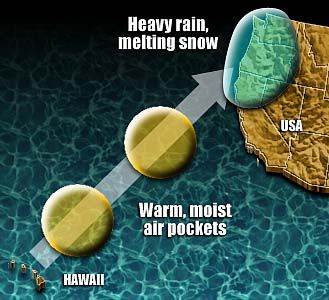
Pineapple Express

PE storms: caused by atmospheric rivers hitting the west
coast in winter

 • Often bring heavy rain and warm temperatures
 • Great impact on water resources of western US

This work aims to answer several questions related to this
phenomenon:

Questions of Interest

1. Are regional climate models, driven by reanalysis, able to
   capture extreme precipitation events associated with PE,
   as seen in observational data? Some previous work: Leung
   and Qian (2009)

2. Can we draw a connection between PE extreme precip-
   itation events and short-lived (daily) synoptic-scale pro-
   cesses?

3. Given a future-scenario climate model run, what might
   extreme precipitation events look like in observations, and
   what is the uncertainty in these estimates?

Method: bivariate extreme value analyses
A statistician’s view

Differing perspectives on climate, weather, and extreme events.

Climate vs. weather: Climate is the distribution of weather
variables like temperature, precipitation, wind, etc.

Extremes: Think of extremes as the upper (or lower) tail of
a distribution; e.g., the very largest values in a time series of
precipitation measurements.

Climate models: Simulate from the distribution of weather
variables over a long period of time (e.g. one year, 5 years,
20 years)
Data and Model Output

We utilize several sources of climate model output and an
observational product:

 • Daily RCM precipitation output from NARCCAP - focus
   on WRF model
 • NCEP/NCAR global reanalysis
 • Daily gridded observational precipitation from University
   of Washington (Maurer et al.)
 • Future run: WRF forced by CCSM global model

We study NDJF days from 1981-1999 (‘current’) and 2041-
2070 (‘future’).
Outline

1. (Very) brief overview of extreme value theory
2. Comparing RCM output extremes to observations
   • Modeling tail dependence
3. “Pineapple Express index”
   • North Pacific SLP fields
4. Examining future Pacific region precipitation extremes
   • Future PE events & uncertainty
5. Summary and Future Work
EVT Approach

The aim of extreme value theory is to describe the (joint)
upper tail of a (multivariate) distribution. It is not necessary
to know the data’s entire distribution.

 • Univariate case: we employ a threshold exceedance ap-
   proach using the Generalized Pareto Distribution:
                                               !−1/ξ
                                         x−u
               P(X > x|X > u) ≈ 1 + ξ
                                          ψu    +

 • ξ determines tail behavior (bounded, light, heavy) and is
   difficult to estimate
 • Bivariate extremes: estimate marginals first, then trans-
   form to unit Fréchet: FZ (z) = exp{−z −1}
 • Tail dependence is described by an angular measure
Radial and angular components
1.0
0.8
0.6
r/t[,2]
r
0.4
0.2
w
0.0
0.0 0.2 0.4 0.6 0.8 1.0
r/t[,1]Comparing WRF model output to observations
We define a study region and quantity with the purpose of
capturing PE events identified by Dettinger et al. (2011).
WRF Obs
250
50
50
200
45
45
150
100
40
40
50
35
35
0
-124 -121 -118 -124 -121 -118
Precipitation from WRF-reanalysis output (left) and observational data product (right) on January 1, 1997.Estimation of marginal tails
GPDs are fit to the largest 5% of data in each margin:
Margin u· ψ̂· (se) ξ̂· (se)
XtN C (WRF) 1054 288.95(39.27) 0.0255(0.104)
YtC (obs) 14240 3895.87(512.03) 0.0213(0.099)
Each margin is transformed to unit Fréchet:
Original Scale Frechet Scale
Pineapple Express Days
2500
30000
Non-PE Days
2000
Observed Precip
Observed Precip
20000
1500
1000
10000
500
0
0
0 500 1000 1500 2000 2500 0 500 1000 1500 2000 2500
WRFG Output WRFG OutputExamining tail dependence
We find tail dependence and fit a parametric model to the
angular density of points with large ‘radial’ components.
Frechet scale Histogram of w for r > r0
200
Logistic model
Dirichlet model
1.5
150
Observed Precipitation
Density
1.0
100
0.5
50
0.0
0
0 50 100 150 200 0.0 0.2 0.4 0.6 0.8 1.0
WRF Output w
+ WRF reproduces extreme events relatively well
− Not all ‘extreme’ events associated with Pineapple Express:
aim to connect to synoptic-scale processesPineapple Express Index
Mean sea-level pressure fields are extracted from the NCEP
reanalysis product
Mean Anomaly on Extreme Precip PE days Mean Anomaly on Extreme Precip non-PE days
60
60
0
55
55
-500
50
50
45
45
-1000
40
40
-1500
35
35
30
30
-150 -140 -130 -120 -110 -150 -140 -130 -120 -110
Composite anomaly fields for largest 130 observed precipitation days, partitioned into PE and non-PE
Define a daily index as a projection onto PE anomaly field -
exhibits tail dependence with precipitationFuture PE Extremes We analyze precipitation output from WRF driven by CCSM global model (2041-2070). • Previous studies suggest increases in frequency and inten- sity of PE under A2. Here: use fitted dependence model and PE index to simulate future observed precipitation extremes, given climate model output Challenges: we need to estimate 1. Marginal distribution of future reanalysis-driven precipita- tion 2. Marginal distribution of future observations
Extremes from the NARCCAP ensemble

Use other NARCCAP model combinations to infer the upper
tail of future reanalysis-driven WRF precipitation:

                        GCM
           RCM CCSM CGCM3 GFDL NCEP
          WRFG   X    X         X
          ECP2              X   X
          CRCM   X    X         X
          MM5I   X              X
          RCM3        X     X   X

 • GCM-driven runs for current and future; reanalysis for cur-
   rent only
 • For each RCM-GCM-time combination, obtain ML esti-
   mates and standard errors of GPD parameters
Estimating future reanalysis-driven WRF
An ‘ANOVA-like’ model on the parameters of the GPD:
! ! ! ! !
ψijr µψ αiψ βjψ γ
= + + + ψ 1{r=2}(r) + ijr
ξijr µξ αiξ βjξ γξ
• αi = effect of RCM i, i = 1, ..., 5
• βj = effect of GCM j, j = 1, ..., 4 (4 = reanalysis)
• γ = difference between current and future
• ijr incorporates numerically estimated covariances
Estimates:
• β̂4ξ = 0.150 ⇒ NCEP-driven RCM runs produce heavier
tail of precipitation than GCM-driven runs
• γ̂ξ = 0.057: evidence for heavier-tailed precipitation in A2
scenario (WRF 100-year event becomes 36.3-year event)Simulation of observations
Repeated simulation gives uncertainty estimates based on
how RCM represents extreme events.
40000
30000
yDat
20000
10000
0
0 500 1000 1500 2000 2500 3000
xDat
x-axis: WRF-CCSM output. y-axis: simulated observationsPE Index of simulated future events
Color shows PE index expressed as a z-score
45000
3
Simulated Precipitation Footprint
35000
2
1
25000
0
-1
15000
2040 2045 2050 2055 2060 2065 2070
Year
Plot shows only observations simulated to be extreme, dashed line corresponds to largest event in current period (1981-
1999)Uncertainty through Simulation
We examine two quantities of interest through simulation:
• q1: Proportion of simulated exceedances of p quantile
which correspond to exceedances of p quantile of PE index
values (p ≈ 0.96).
• q2: Proportion of ‘extreme’ observations occurring in years
2055-2070 (measure of nonstationarity)
Quantity Estimate1 95% Interval1
q1 0.203∗ (0.144, 0.257)
q2 0.571 (0.477, 0.656)
1 Based on 500 conditional simulations
∗ Value from current period: 0.143
Evidence for increased correspondence of PE events and ex-
treme precipitation - more intense PE eventsSummary This work is a novel application of bivariate EVT in a climate study. • Tail dependence between RCM output and observations - modeled this parametrically • PE Index - derived from SLP fields; tail dependent to observed precipitation • Conditional simulation from parametric model given future RCM output - uncertainty estimates
Future work

Important to remember that we have studied one RCM,
driven by one GCM, and compared it to one observational
product.

 • Improvement of the PE index - storms evolve over several
   days
 • PE events from other climate models
 • Examining other regions/phenomena
Reference

Manuscript and figures available at
http://www.stat.colostate.edu/~weller.

References

Dettinger, M., Ralph, F., Das, T., Neiman, P., and Cayan, D.
 (2011). Atmospheric rivers, floods and the water resources
 of California. Water, 3(2):445–478.
Leung, L. and Qian, Y. (2009). Atmospheric rivers induced
 heavy precipitation and flooding in the western US simulated
 by the WRF regional climate model. Geophysical Research
 Letters, 36(3):L03820.
Weller, G., Cooley, D., and Sain, S. (2012). An investigation
 of the Pineapple Express phenomenon via bivariate extreme
 value theory. Environmetrics.
You can also read