ANALYSIS AND MODEL DEVELOPMENT OF DIRECT HYPERSPECTRAL CHLOROPHYLL-A ESTIMATION FOR REMOTE SENSING SATELLITES
←
→
Page content transcription
If your browser does not render page correctly, please read the page content below
ANALYSIS AND MODEL DEVELOPMENT OF DIRECT HYPERSPECTRAL
             CHLOROPHYLL-A ESTIMATION FOR REMOTE SENSING SATELLITES

                                   Sivert Bakken1 , Geir Johnsen2 , Tor A. Johansen 1

                              Center for Autonomous Marine Operations and Systems
                                   Department of Engineering Cybernetics(1) &
                                            Department of Biology(2)
                             Norwegian University of Science and Technology (NTNU)
                                               Trondheim, Norway

                         ABSTRACT                                   (CDOM), and Total Suspended Matter (TSM) that confound
                                                                    the model [3].
The advancement of instruments makes processing of hyper-
                                                                        Nonlinear machine learning methods, e.g. Neural Net-
spectral data for monitoring phytoplankton dynamics more
                                                                    works (NN) or kernel-based regression models such as Gaus-
viable. Methods used operationally for retrieval of chl-a, an
                                                                    sian Process Regression (GPR) and Support Vector Machines
important indicator of phytoplankton, are developed for mul-
                                                                    (SVM), can give good chl-a estimations, but will also have
tispectral systems and optically deep waters. Coastal waters
                                                                    a higher level of complexity [4]. The relative relevance of
are important for the aquaculture industry, marine science,
                                                                    the input features is less transparent, it is more challenging
and environmental monitoring. Data rate limitations make the
                                                                    to foresee the model behavior by theoretical analysis, and
use of sensors with high spectral resolution difficult. Here, es-
                                                                    the models themselves will be computationally more demand-
timation of chl-a from top of the atmosphere reflectance using
                                                                    ing to use for estimation when compared to linear prediction
“Partial Least Squares”- and “Least Absolute Shrinkage and
                                                                    models [3, 4, 5]. However, for any linear model, nonlin-
Selection Operator”-regression is compared with the internal
                                                                    ear patterns can be compensated for by the appropriate pre-
consistency of the OC4 algorithm by NASA Ocean Biology
                                                                    processing or by kernel functions [6].
Processing Group.
                                                                        Partial Least Squares Regression (PLSR) has been demon-
    The models perform better in terms of NRMSE and R2
                                                                    strated to perform with greater accuracy than optimized band
when validated with a subset of the total data and with a sepa-
                                                                    ratio algorithms when predicting chl-a concentrations with
rate scene. This is demonstrated by using experimental hyper-
                                                                    field-retrieved hyperspectral water-leaving reflectance [3].
spectral scenes from the Hyperspectral Imager for the Coastal
                                                                    Hyperspectral water-leaving reflectance values are depen-
Ocean (HICO) mission, processed through SeaDAS.
                                                                    dent on an accurate atmospheric correction[2, 7]. This can
   Index Terms— Hyperpsectral Imaging, Remote Sensing,              be difficult to achieve in coastal regions, and hyperspectral
Chlorophyll-a Concentration, Ocean Color                            atmospheric correction for ocean color is an active area of
                                                                    research [7, 8, 2].
                                                                        In this paper, different approaches to perform regression
                    1. INTRODUCTION
                                                                    analysis and model development using top-of-the-atmosphere
                                                                    reflectance values from the hyperspectral image data from the
The study of Ocean Color has many potential societal benefits
                                                                    HICO mission are used to estimate the chl-a concentration.
[1]. Chl-a concentration monitoring can provide the aquacul-
                                                                    The chl-a concentration is computed by SeaDAS. The results
ture industry and the government information regarding wa-
                                                                    from the regression are then compared to the OC4 band-ratio
ter quality, biogeochemical cycles, and fisheries management.
                                                                    algorithm.With the demonstrated approach the PLSR mod-
For research, the chl-a concentration provides a bio-marker
                                                                    els developed are intuitively interpretive, less computation-
for the state of the marine ecosystems, as well as an aid to
                                                                    ally demanding, and generate promising results. Shown with
modeling the ocean state and monitoring climate change.
                                                                    different designs for validation.
    With traditional band-ratio algorithms for chl-a estima-
tion, like OC4, it has been shown that additional spectral
information improves the results [2]. Successful application                     2. HICO DATA AND SEADAS
of band-ratio algorithms in optically complex waters is of-
ten challenging due to overlapping of spectral signals from         The Hyperspectral Imager for the Coastal Ocean (HICO) mis-
phytoplankton (chl-a), Colored Dissolved Organic Matter             sion was a hyperspectral instrument onboard the International
Training Data
Space Station capable of capturing scenes with 128 different
wavelengths in a range from 350 to 1080 nm at a 5 nm reso- 6
Training Chlorphyll
lution [9]. 5
4
Here, hyperspectral scenes from the HICO mission, pro-
3
cessed and quality controlled through NASA OBPG software
2
SeaDAS, are used as the desired values for chl-a. The re-
1
flectance data used is derived from the standard atmospheric
0
correction provided by SeaDAS for HICO. 0 1000 2000 3000 4000 5000
Sample number
Verification Data
6
Verification Chlorphyll
5
4
3
2
1
0
0 500 1000 1500 2000
Sample Number
Fig. 2: Chl-a concentrations for the sampled data
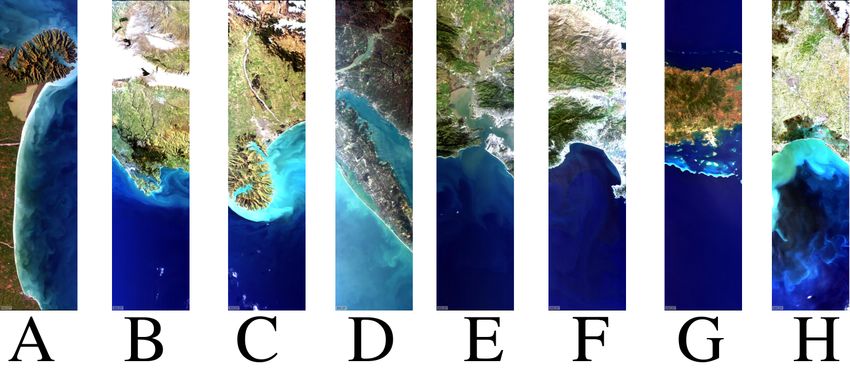
Fig. 1: HICO Sample Image Gallery Scenes from different
locations around the world used for training and validation.
reported as noisy [9]. No preprocessing in terms of dimen-
The scenes were selected due to the low adverse effects sionality reduction has been performed.
from atmospheric interference and good overall imaging qual- Top-of-atmosphere reflectance ρ(λ), can be defined at a
ity from the HICO Sample Image Gallery [10]. The scenes given wavelength λ, to be related to the radiance L(λ), the ex-
can be seen in figure 1 and their locations are, from the left, traterrestrial solar irradiance F0 (λ), and the solar-zenith angle
southeast coast of New Zealand (A-C), US west coast (D-F), θ0 , as given in equation (1) [7].
New Caledonia, and Italy.
The chl-a concentrations in mg/m−3 for the training and ρ(λ) = πL(λ)/(F0 (λ) cos(θ0 )) (1)
the verification data sets are displayed in Figure 2. The HICO First, with the assumption that the variations in F0 (λ) are
chl-a data used as ground truth are derived through SeaDAS small compared to the sun angle effects, the reflectance values
which, as standard, used the OC4 algorithm with MERIS co- are approximated as ρ̂(λ) by dividing the radiance data with
efficients and wavelengths [11]. In SeaDAS, the hyperspec- the solar zenith angle.
tral data is subsampled to the MERIS bandwidths when deriv- Secondly, the effect of attenuation of light is accounted for
ing chl-a. From each scene, 700 sample spectra are taken for by computing the log values of the approximated reflectances
training, and 300 different spectra are taken for verification in as ρ̃(λ) = log10 (ρ̂(λ))[12].
the initial validation procedure. In the secondary validation Finally, the input variables have been centered and scaled
procedure, the fourth scene from the left, scene D, in Figure to adhere to different absolute values and variation for a given
1 is kept out and only used as a validation data set, as it has a wavelength [5]. This is given in equation (2), where x̂ is the
good dynamic range. See section 4 for details about the val- new variable, ρ̃(λ) is the old, ρ̄(λ) is the mean, and σρ is the
idation procedures. The chl-a concentration for each sample standard deviation.
can be seen in Figure 2 for the first validation procedure.
ρ̃(λ) − ρ̄(λ)
x̂ = (2)
σρ
3. METHODS
3.1. OC4 by NASA OBPG
A conceptual description of the different algorithms and their
advantages and shortcomings are presented. A complete The OC4 algorithm developed by NASA OBPG [11], pre-
derivation of the algorithms is beyond the scope of this paper, sented in equation (3), returns the near-surface concentration
but references are provided. of chl-a in mg/m−3 . The algorithm uses an empirical re-
The preprocessing of the input variables in this paper in- lationship derived from in situ measurements of chl-a con-
corporates known physical relationships [5]. Only the radi- centration and corresponding above-water remote sensing
ance signals from 400 to 900 nm are used, which leaves 87 reflectances Rrs , with 4 spectral bands [2]. In this paper,
spectral bands. The wavelengths outside this range have been the implementation of the OC4 algorithm uses the spectralbands closest to the ones used by the SeaWiFS multispectral 4.1. OC4 Algorithm
imager[13, 2]. Rrs (λgreen ) is the band closest to 555 nm, and
Rrs (λblue ) is the maximum of the bands closest to 443, 490, The ai coefficients used in equation (3) for the OC4 is com-
or 510 nm. The ai coefficients used in the implementation of puted by taking the least-squares fit of the training data set.
OC4 presented here were found using ordinary least squares This should give OC4 the best possible starting point.
on the training data presented in Figure 2 [5]. As can be seen in Figure 4 the OC4 algorithm performs
similar to previously reported tests [2, 11]. With validation
using a subset of the total data i.e. the verification data set
4 i no clear trend in the residuals can be found. The algorithm
X Rrs (λblue )
log10 (chl a) = ai log10 (3) struggles to determine chl-a > 4mg/m3 , with the coefficients
i=0
Rrs (λgreen )
found.
For the validation with a separated scene, scene D in Fig-
3.2. Partial Least Squares ure 1, the OC4 algorithm can determine a qualitative chl-a
concentration within a given scene from SeaDAS, but is not
Partial least-squares regression (PLSR) iteratively relates able to quantify it accurately.
data matrices using linear multivariate models that reduce
collinearity and noise within a given dataset. It is a two-step LASSO Coefficient Plots
algorithm that first finds uncorrelated components in the vari-
2
ables of a given data set and then performs the least squares
Coefficient Value
regression on these components. A more in-depth description 0
of the algorithm can be found in [14].
-2
This generates models with high levels of interpretabil-
ity, but in their simplest form cannot accommodate for strong -4
400 500 600 700 800 900
nonlinear effects[5]. Wavelength (nm)
PLSR Coefficient Plots
4
3.3. Least Absolute Shrinkage and Selection Operator
Coefficient Value
2
Least Absolute Shrinkage and Selection Operator (LASSO) 0
regression [15] was performed using the approach found in -2
equation (4), where yi is chl-a values, βi is the regression -4
coefficients, X is a matrix with all the pre-processed data,
400 500 600 700 800 900
and t is a threshold that was iterated over with 10-fold cross- Wavelength (nm)
validation of the training data. The threshold that gave the
lowest mean square error was selected. Fig. 3: Regression coefficients from PLSR and LASSO
This also generates models with high levels of inter-
pretability, but in their simplest form cannot accommodate
strong nonlinear effects. This method does not seek to find
4.2. Regression Models
any covariation between variables. A vector of all ones is
represented as 1N . LASSO and PLSR are both linear regression models that pro-
vide interpretable coefficients, as can be seen in Figure 3. The
models developed deployed 10-fold cross-validation with the
2
min k(yi − β0 1N − Xβk2 s.t. kβk1 ≤ t (4) training data set when determining the weights of the regres-
β0 ,β
sion. For the PLSR the average mean square error from the
10-fold CV was used to select the number of components, i.e.
4. RESULTS & DISCUSSION 20 components, to be used in the regression.
As can be seen in Figure 4, both the LASSO and PLSR
Presented in this section is a discussion comparing the results models perform similarly on the given data set. From the
in terms of regression coefficients, Normalized Root Mean results, PLSR has a potentially negligible higher performance
Square (NRMSE) and R-squared (R2 ) values for OC4, PLSR in terms of NRMSE and R-squared when compared with
and LASSO. LASSO. It should be noted that LASSO here uses 67 of
All models were tested with the verification data set the original 87 variables, which can be valuable from an
shown in Figure 2, as well as separating out the fourth scene operational point of view in terms of execution time. The
from the left in Figure 1, scene D as the scene inhibits a good regression models also struggle to determine higher chl-a.
dynamic range in terms of chl-a. Possibly, due to lack of data or non-linear effects.PLSR Validated Using Subset of Data LASSO Validated Using Subset of Data OC4 Validated Using Subset of Data
7 7 7
2
R : 0.9665 2
R : 0.9654 R2 : 0.8439
NRMSE: 0.1832 NRMSE: 0.1862 6 NRMSE: 0.3976
6 6
5
Estimated Chlorophyll-a
5 5
Estimated Chlorophyll-a
Estimated Chlorophyll-a
4 4 4
3 3 3
2 2 2
1 1 1
0 0 0
0 1 2 3 4 5 6 7 0 1 2 3 4 5 6 7 0 1 2 3 4 5 6 7
SeaDAS Chlorophyll-a SeaDAS Chlorophyll-a SeaDAS Chlorphyll-a
PLSR Validated With Scene D LASSO Validated Using Scene D OC4 Validated Using Scene D
6 7 7
R2 : 0.9439 2
R : 0.9363 R2 : 0.9296
NRMSE: 0.4270 NRMSE: 0.4491 NRMSE: 0.7546
6 6
5
5
Estimated Chlorophyll-a
5
Estimated Chlorophyll-a
Estimated Chlorophyll-a
4
4 4
3
3 3
2
2 2
1
1 1
0 0 0
0 1 2 3 4 5 6 0 1 2 3 4 5 6 7 0 1 2 3 4 5 6 7
SeaDAS Chlorophyll-a SeaDAS Chlorophyll-a SeaDAS Chlorophyll-a
Fig. 4: Results from scenes showing Normalized Root Mean Square and R squared.
For the validation with a separated scene, scene D in Fig- models perform better than the OC4 algorithm in terms of
ure 1, the regression models are also able to determine a rela- NRMSE and R-squared for the used validation schemes. The
tive and more accurate quantification of the chl-a. The regres- two regression models have a similar performance in terms
sion models have a better performance to the OC4 algorithm of the chosen metrics, but the execution time of the LASSO
with the validation scheme using data from all scenes. regression was on average 1.8 times faster.
From the coefficient illustrated in Figure 3, it is clear that
4.3. Comparison the LASSO and PLSR approach puts emphasis on similar
parts of the electromagnetic spectrum. It is also clear that
It should be noted that this is a test of the internal consistency some of the coefficients, > 555 nm and < 443 nm, have high
of OC4 within the SeaDAS software, i.e. how different bands expressive power in terms of determining the total chl-a con-
used as a basis for OC4 will perform. A more proper data set centration. The wavelengths 555 nm and 443nm indicate the
with ground-truth samples measured by other means would maximum and minimum of the OC4 algorithm. That addi-
be a better study, and could even yield an even higher per- tional spectral information improves chlorophyll determina-
formance increase with the approach given in this paper. The tion, and this corresponds well with other findings investigat-
approach used here should benefit the OC4 algorithm. ing band-ratio algorithms [2].
With the preprocessing described in section 3 the vari-
ables are an atmospheric correction and a 4th order polyno-
mial kernel [6] from having the same form as equation (3). 5. CONCLUSIONS & FUTURE WORK
The data representation chosen for regression incorporates
a well-characterized non-linear physical relationship, e.g. The presented machine learning models seem may provide
transformation from radiance to reflectance and light attenu- absolute measurements of chl-a concentration from only us-
ation. This ensures that the machine learning algorithms, i.e. ing the measured top-of-the-atmosphere radiance, the attitude
different forms for regression, do not put a lot of emphasis on and solar angle information related to the hyperspectral sen-
estimating non-linear relationships. sor.
As can be seen in Figure 4, both the LASSO and PLSR Multivariate methods such as PLSR seems to be suitablefor deriving some geophysical variables of interest such as [5] Kristin Tøndel and Harald Martens, “Analyzing com-
chlorophyll-a concentration. At the same time, these linear plex mathematical model behavior by partial least
methods can provide an interpretable derivation of results in squares regression-based multivariate metamodeling,”
the form of coefficients. This makes it easier to understand Wiley Interdisciplinary Reviews: Computational Statis-
why the models derive the values that they do, which in return tics, vol. 6, no. 6, pp. 440–475, 2014.
can provide reassurance to the end-user.
[6] Bernhard Scholkopf and Alexander J Smola, Learning
The LASSO model, when compared to PLSR, provided a
with kernels: support vector machines, regularization,
reduction to 54% in the average computational time per pixel,
optimization, and beyond, MIT press, 2001.
encourages its use in computationally constrained systems.
These results are implementation and hardware dependent. [7] IOCCG, Atmospheric Correction for Remotely-Sensed
When doing machine learning there is a considerable ad- Ocean-Colour Products, vol. No. 10 of Reports of
vantage of having large data sets with verified ground truth, the International Ocean Colour Coordinating Group,
but this is not widely available for hyperspectral ocean color IOCCG, Dartmouth, Canada, 2010.
remote sensing data, thus HICO data quality assured through
SeaDAS was used. When more ground truth data become [8] Amir Ibrahim, Bryan Franz, Ziauddin Ahmad, Richard
available with future space missions and systems, better mod- Healy, Kirk Knobelspiesse, Bo-Cai Gao, Chris Proctor,
els could be developed using this approach. Also, the data and Peng-Wang Zhai, “Atmospheric correction for hy-
used in this paper does only represent a subset of the full perspectral ocean color retrieval with application to the
range of naturally occurring chlorophyll-a concentrations. hyperspectral imager for the coastal ocean (hico),” Re-
With more data, better models could be developed. mote Sensing of Environment, vol. 204, pp. 60–75, 2018.
Preprocessing with targeted binning of spectral regions of [9] Robert L Lucke, Michael Corson, Norman R McGloth-
interest for chlorophyll-a concentration, found through analy- lin, Steve D Butcher, Daniel L Wood, Daniel R Kor-
sis of the regression coefficients, could improve the signal to wan, Rong R Li, Willliam A Snyder, Curt O Davis, and
noise ratio of the spectra and in return improve the estimation Davidson T Chen, “Hyperspectral imager for the coastal
performance, and should thus be further investigated. ocean: instrument description and first images,” Applied
optics, vol. 50, no. 11, pp. 1501–1516, 2011.
6. ACKNOWLEDGEMENTS [10] “Hico - sample image gallery,” http:
//hico.coas.oregonstate.edu/gallery/
This work was supported by the Norwegian Research Council gallery-scenes.php, (Accessed on 04-02-2020).
through the Centre of Autonomous Marine Operations and
Systems (NTNU AMOS) (grant no. 223254), the MASSIVE [11] “Nasa ocean color,” https://oceancolor.
project (grant no. 270959). gsfc.nasa.gov/atbd/chlor_a/, (Accessed on
03-03-2020).
7. REFERENCES [12] Howard R Gordon, “Can the lambert-beer law be ap-
plied to the diffuse attenuation coefficient of ocean wa-
[1] Trevor Platt, Why ocean colour?: The societal benefits ter?,” Limnology and Oceanography, vol. 34, no. 8, pp.
of ocean-colour technology, Number 7 in IOCCG re- 1389–1409, 1989.
ports. International Ocean-Colour Coordinating Group,
2008. [13] John E O’Reilly, Stephane Maritorena, B Greg Mitchell,
David A Siegel, Kendall L Carder, Sara A Garver, Mati
[2] John E O’Reilly and P Jeremy Werdell, “Chlorophyll Kahru, and Charles McClain, “Ocean color chlorophyll
algorithms for ocean color sensors-oc4, oc5 & oc6,” Re- algorithms for seawifs,” Journal of Geophysical Re-
mote sensing of environment, vol. 229, pp. 32–47, 2019. search: Oceans, vol. 103, no. C11, pp. 24937–24953,
1998.
[3] Kimberly Ryan and Khalid Ali, “Application of a partial
least-squares regression model to retrieve chlorophyll- [14] Svante Wold, Michael Sjöström, and Lennart Eriks-
a concentrations in coastal waters using hyper-spectral son, “PLS-regression: a basic tool of chemometrics,”
data,” Ocean Science Journal, vol. 51, no. 2, pp. 209– Chemometrics and intelligent laboratory systems, vol.
221, 2016. 58, no. 2, pp. 109–130, 2001.
[15] Robert Tibshirani, “Regression shrinkage and selection
[4] Katalin Blix and Torbjørn Eltoft, “Machine learn- via the lasso,” Journal of the Royal Statistical Society:
ing automatic model selection algorithm for oceanic Series B (Methodological), vol. 58, no. 1, pp. 267–288,
chlorophyll-a content retrieval,” Remote Sensing, vol. 1996.
10, no. 5, pp. 775, 2018.You can also read