Analysis of Amazon Stock Using Simple Linear Regression and Time Series ARIMA Model

Highlights in Science, Engineering and Technology TPCEE 2022
Volume 38 (2023)

 Analysis of Amazon Stock Using Simple Linear Regression
 and Time Series ARIMA Model
 Xiaoyu Ma*
 Department of Statistical Science, University of Toronto, Toronto, Canada
 *Corresponding author: xiaoy.ma@mail.utoronto.ca
Abstract. The rate of daily return of a stock is one of the important indicators for investors to
anticipate benefits or losses from historical data. This paper will focus on the stock of Amazon, which
is a popular choice for stock traders and contains data from August 25, 2017, to August 24, 2022.
By using regression models such as a simple linear regression model and an autoregressive
integrated moving average (ARIMA), the recent daily return value is predicted based on data during
these 5 years. The simple linear regression can show the trend of stock price and the predicted
response rate of daily return using the linear model. Furthermore, ARIMA is a more advanced time
series model to provide a more accurate rate of daily return with confidence intervals. The predicted
trend and rate of daily return are useful for investors to make decisions to buy or sell a stock recently.
The trend can tell investors whether the stock price would go up and the daily return can indicate
how many benefits can they earn if they choose to invest in this stock.
Keywords: Amazon, Stock, Daily Return, ARIMA, Simple Linear Regression.

1. Introduction
1.1. Background
 Analysis of a stock is meaningful for stock traders in both long and short positions to make a better
decision based on the known information, for example, historical stock price. However, there are
many issues that can affect the stock price within a short period of time such as news about the
companies, demands for a resource and traders’ sentiment. Therefore, it is not easy to provide an
accurate prediction of the price of a stock along with other important indicators using all the existing
data due to the time-based, complex and fluctuating stock market.
1.2. Related Research
 Forecasting market stocks is a valid judgment of the future value of a company's stock or a
financial product [1], and this judgment can provide a certain probability guarantee of the profit that
will be made with the stock in the end. Currently, linear and nonlinear models are commonly used
for stock price forecasting for time series data. Regarding the linear models, the opening price, highest
price, lowest price and close price of the day can be used to predict stock value [2] but also time can
be used as an independent variable to forecast the value of the stock. The data can then be separated
into a training set and a testing set. In addition, the testing set is used to validate the models built
based on data from the training set [3].
 The linear regression model and data validation can predict stock price, however, due to the
volatility and complexity of the market, forecasting stocks by a single model is not sufficient [1].
Therefore, some scholars believe that integrating various single models for stock forecasting can
somewhat increase the probability of accurate prediction [1], and news mining using text mining
techniques [4]. In addition, the Moving Average (MA) is frequently used to predict stock pricing
related to time series analysis. It is a tool that indicates the average price of a financial asset during a
period and provides a smooth trend for the price of the asset [5]. In particular, Simple Moving
Average (SMA), Exponential Moving Average (EMA) and Weighted Moving Average (WMA) have
concepts related to moving average strategy. Particularly, no matter where the point is found in the
series, each of them in the time series data has the same weight in the SMA model. [6]. The

 353

Highlights in Science, Engineering and Technology TPCEE 2022
Volume 38 (2023)

decomposition also separates the time series into its constituent components to help predict [7]. In
particular, non-seasonal data can decompose using SMA graphs while seasonal time series need to
use some functions to help visualize and adjust [7]. Finally, one more advanced tool that would be
touched on in the research is an autoregressive integrated moving average (ARIMA) combining
autoregressive (AR), I (Integrated), and moving average (MA) models. This method focuses on
autocorrelation issues instead of trend and seasonality only [8, 9]. Moreover, the time series in this
model need to be stationary [7]. Then, with help of ACF and PACF plots, the final ARIMA model
can be selected and interpreted. The normality of forecast error should be checked and the histogram
of residuals should have a mean of zero with a variance of one [7].
1.3. Motivation and Framework
 Most linear regression models that are used to predict stock price are mainly based on historical
data including open price, close price or volume. Although the basic linear models can demonstrate
trends and the rate of change easily, it is not enough to obtain an accurate prediction due to the features
stock market and there are more variables regarding stock that should be considered. The paper will
present the dataset and its variables collected from Yahoo Finance first, following the visualizations
of the data and a brief introduction of regression models. Next, the procedures and results regarding
regression models would be explained clearly. Specifically, the regression models contain a simple
linear regression model and ARIMA. Since noticeable the drawbacks of simple linear regression
models with poor predictions are noticeable, the original data is also trained to test the performance
of this model. In the ARIMA part, there are three parameters needed to be found by human selection
based on graphs and test results. After the parameters are selected, the ARIMA model can be
constructed and the prediction is shown. Finally, the paper would combine two results from simple
linear regression and ARIMA to draw some useful conclusions and suggestions for investors who are
interested in Amazon.

2. Methods
2.1. Source of Data
 The dataset is downloaded from the website Yahoo Finance [12] that contains seven variables
named Date, Open which corresponds to the open price of Amazon’s stock on a specific day, High
which corresponds to the highest price of Amazon’s stock on the same day, Low which corresponds
to the lowest price, Close which corresponds to the close price, Adjusted Close which calculated
using split and dividend multipliers [13] and Volume which is the number of traded shares in a day
[14], and a total of 1258 observations from August 25, 2017, to August 24, 2022. In particular, except
for the variable Date, Open, High, Low, Close, Adjusted Close and Volume are numeric variables.
2.2. Dependent and Independent Variables
 According to the topic that the paper is addressing, the numeric dependent variable is DailyReturn,
which is the per cent of the daily return of Amazon. The independent variable in regression models
such as simple linear regression model and ARIMA model is Date.
2.3. Machine Learning Models
2.3.1 Simple Linear Regression Model
 A linear regression model is one of the simple ways of supervised learning that is practical for
quantitative response prediction [15]. In addition, the model can not only show the association
between the response variable and predictor variables, but also the strength of association. In this
research, there is only one predictor variable Date, then the model would be simple linear regression.
The general formula for a simple linear regression is
 = 0 + 1 1 + ⋯ + + (1)

 354

Highlights in Science, Engineering and Technology TPCEE 2022
Volume 38 (2023)

 Meaning that the response value equals predictor variables plus an error term [16]. In this research,
the model is
 = 0 + 1 1 + (2)
 Where is the predicted rate of daily return, 0 is the interception, 1 is the rate of change of
daily return in percentage, 1 is the number of days after August 25, 2017, and is the error term.
Meanwhile, there are some assumptions of linear regression models that should be checked and
satisfied (e.g., linear relationship, independent errors, normal errors and homoscedasticity) before
estimating the accuracy of these coefficients and the model.
 The evaluation of a model, or to say the performance of the model to explain the rate of daily
return using predictor variable Date can be determined by adjusted R squared and p-value based on
in-sample data. Since there is no evidence or information to indicate how well the model can predict
some new data, then eighty per cent of observations from the original dataset is split into training data
sets and the left is assigned to a testing set. Based on the root-mean-square error (RMSE), the
performance of the testing model will be evaluated, which shows how well the linear model can
explain new data, or to say, how well the model predicts the percentage of daily return outside the
time frame from August 25, 2017, to August 24, 2022.
2.3.2 Time series Analysis – ARIMA
 The other regression model approach regarding time series data is ARIMA which is commonly
utilized to forecast capital market and stock price [4]. It is a model that can regress on previous
changing values (AR), differencing observations to have a stationary time series (I) and show the
relationship between an observation and past error (MA) [9]. In particular, the parameter of AR model
is p which is the order of the autoregressive part, the one of MA model is q showing the order of the
moving average part and I model’s parameter is d equals to the degree of first differencing involved
[9]. Before constructing an ARIMA model, the stationary variable should be checked first using the
Augmented Dickey-Fuller unit root test since ARIMA requires time series is stationary with constant
mean and variance. Then differencing the variable to be stationary, if needed. Meanwhile, if the
variable is stationary then the d value is 0, otherwise, the d value equals the number of times of
differencing to stationary status. Next, the parameter p in AR and the parameter q in MA can be found
using auto-correlation graph (ACF) and partial auto-correlation graph (PACF) graphs, respectively,
so that the best model has the lowest AIC or BIC value. To be specific, ACF is the correlation between
each observation and the previous ones with a lag of the number of time points between in an ACF
plot while PACF shows the correlations between the current ones and the previous one that can not
be explained by correlation using lower order lags [8]. After the parameters p, q, and d are selected,
an ARIMA model can be built. The prediction is provided along with 80% and 90% confidence
intervals. Finally, after the best model is found, the normality of residuals is needed to be checked to
ensure the selected model is white noise [8].

3. Methods
3.1. Data Processing
3.1.1. Variables and Observations
 The dataset is downloaded from the website Yahoo Finance [13] that contains seven variables
named Date, Open, High, Low, Close, Adjusted Close and Volume, and a total of 1258 observations
from August 25, 2017, to August 25, 2022. Except for the variable Date, Open, High, Low, Close,
Adjusted Close and Volume are numeric variables. The variable Date is changed to a date variable
for coding purposes. In addition, a new numeric variable named DailyReturn is added to the dataset
since the research aims to learn about the percentage of returns and the trend of Amazon stock prices
over a period of time (e.g., 5 years in this paper) to predict future daily return and arbitrage
opportunities. Specifically, the daily return has calculated the difference between today’s close value

 355

Highlights in Science, Engineering and Technology TPCEE 2022
Volume 38 (2023)

and yesterday's close value. Therefore, the dataset now has one date variable and seven numeric
variables with 1257 observations since the missing value is dropped after a new variable is added.
3.1.2. Training and Testing Sets
 The original data set is divided into a training set and a testing set for evaluation of simple linear
regression model performance purpose. Therefore, the training set contains 80% of observations from
the original one while the testing set has 20% of observations. The observations assign to groups
randomly. The evaluation will be discussed in section 3.3.1.
3.2. Data Visualization

 Fig. 1 Histogram for price of Open, High, Low and Close of Amazon in last 5 years.
 Photo credit: Original
 Fig. 1 contains four histograms which demonstrate that the open, high, low and close prices from
August 25 2017 to August 24 2022. It shows that the graphs are similar for all price types with two
peaks around 90 and 160. In other words, the stock price has been concentrated at approximate 90
dollars or 160 dollars per stock, which emphasizes an obvious change in the stock price during the
last five years. Meanwhile, it is noticed that the mean stock prices for Open, High, Low and Close
are around 115 dollars per stock. Specifically, the mean close stock price is 116.10 dollars per stock.

 Fig. 2 Scatter plot for price of Open, High, Low and Close of Amazon in last 5 years with linear
 regression.
 Photo credit: Original

 356

Highlights in Science, Engineering and Technology TPCEE 2022
Volume 38 (2023)

 Fig. 2 contains four scatter plots which demonstrate the trends of open, high, low and close prices
respectively from August 25 2017 to August 24 2022. It shows that the prices are increasing by time
for all price types.

 Fig. 3 Daily return in percentages.
 Photo credit: Original
 A new numeric variable DailyReturn is added to the original dataset due to the aim of this paper.
As shown in Fig. 3 above, the percentage of daily return during these years has no apparent changes
and with a mean of 0.1061 per cent. Fig. 3 also shows that the variable is stationary.
3.3. Simple Linear Regression
3.3.1. Analysis of Results from Linear Regression
 Table 1. Coefficients and P-value from R results
 Coefficients Estimate Standard Error t value P value
 Intercept 2.9427507 2.1213671 1.387 0.166
 Date -0.0001549 0.0001158 -1.388 0.181

 As shown in Table 1, the simple linear regression model is
 DailyReturn = 2.9428 − 0.0002 ∗ Date (3)
 Based on the results calculated in R. Therefore, starting from 2.9428% of daily return at the
beginning of 2017, the percentage was predicted to decrease by 0.0002 per cent each day.
3.3.2. Evaluating the Simple Linear Regression
 Table 2. Evaluation of Simple Linear Regression
 Adjusted R-squared p-value
 0.0006282 0.1812

 Based on Table 2, the adjusted R-squared of this model is 0.0006, which means that only a small
part of the variability of daily return can be explained by Date, which shows that simple linear
regression is not a practical way to predict. The RMSE (root-mean-square error) is 2.16.

 357

Highlights in Science, Engineering and Technology TPCEE 2022
Volume 38 (2023)

3.3.3. Assumptions of Linear Regression Models

 Fig. 4 Plots for checking linear regression assumptions
 Photo credit: Original
 Since there is no apparent pattern and all the residuals are randomly distributed around the centre
line of zero on the top left graph in Fig. 4, then the linearity of the model and errors' independence
are satisfied. The top right Q-Q plot in Fig. 4 indicates the normality and it seems that many points
do not lie on the point line in the graph so the normality may not satisfy. Furthermore, the bottom left
graph in Figure 4 demonstrates the assumption of constant variance. It is found that most of the points
are within a certain interval, hence, the assumption is met. However, it is noticeable that there are
some outliers and leverage points in the data set.
3.3.4. Train the data and Evaluate the Performance
 The observations are randomly split into a training set and a testing set where the training set
obtains 80% of observations from the original data. The same linear model with predictor variable
Date and response variable DailyReturn is built using data and information from the training data set.
Then using the model from the training data set to predict the model for testing data but using
information from the testing data set. The RMSE of the testing model is 2.42, which is a little greater
than the one in the original data. This can be explained by the data and information that have not been
observed before. Therefore, the linear regression model is not “good”.

 358

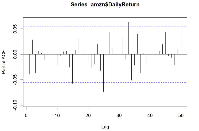
Highlights in Science, Engineering and Technology TPCEE 2022
Volume 38 (2023)

3.4. Time series model – ARIMA
3.4.1. Check Stationary using Dickey-Fuller Test and Find d value

 Fig. 5 Differencing the data to achieve stationarity.
 Photo credit: Original
 The time series data looks stationary since the p-value 0.01 is less than alpha level 0.05, then there
is no evidence to reject the null hypothesis. Therefore, the time series is stationary and the variable is
not needed to be stationaized later. Meanwhile, since there is no differencing occurs, then the d value
in ARIMA is 0. Fig. 5 also shows that the variable is stationary that centered at 0.
3.4.2. p and q values using ACF and PACF
 There is no significant spike or strong correlation after a lag of 0 in ACF graph as shown in Fig.
6, then the model is MA (0).
 From Fig. 7, there is no significant spike in the first few lags in this PACF plot, then it is AR (0).
Figure 6 and Fig. 7 also show that there is no obvious pattern within lags interval, then it seems that
the data does not have seasonal components, which can be demonstrated by simple moving average
graph in Fig. 8 to decompose non-seasonal time series data.

 Fig. 6 Plot of ACF
 Photo credit: Original

 359

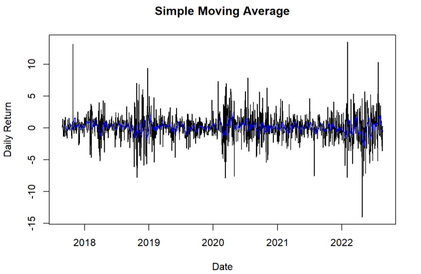
Highlights in Science, Engineering and Technology TPCEE 2022
Volume 38 (2023)

 Fig. 7 Plot of PACF
 Photo credit: Original

 Fig. 8 Graph of Simple Moving Average
 Photo credit: Original
 From Fig. 8, it demonstrates that the time series is non-seasonal again by decomposing using
simple moving average graph, which can estimate the component of trend in additive model.
 According to the findings and conclusions from ACF and PACF graphs, ARIMA with p, d, q equal
to 0 can be tested. On the other hand, there is another simple way to find p, d, q values of the model,
which is auto.arima() function in R. Based on the results from auto testing, the same p, d, q values
are gathered so the model has the lowest AIC value now.
3.4.3. Fit an ARIMA model
 Using ARIMA (p=0, d=0, q=0), the rate of daily return is predicted as the blue line shown in the
Fig. 9, with the 80% confidence interval with color of dark grey, and the 95% confidence interval
with color of light grey. The mean of daily return prediction is 0.1062 per cent with AIC of 5508.41
and RMSE of 2.16. Hence, the future daily return of Amazon stock should be around 0.1 per cent,
and there is 80% of confidence to say the future daily return is within -3% to 3% and 90% of
confidence to say the return is within -4% to 4%.

 360

Highlights in Science, Engineering and Technology TPCEE 2022
Volume 38 (2023)

Fig. 9 Prediction of daily return with 80% confidence interval with color of dark grey and the 95%
 confidence interval with color of light grey.
 Photo credit: Original
3.4.4. Normality of residuals

 Fig. 10 Histogram for checking assumption of normality of residuals.
 Photo credit: Original
 Finally, the normality of forecast errors is checked by plotting a histogram. From Fig. 10, the
distribution of forecast errors is normal, the mean of zero and constant variance are demonstrated as
well. Thus, this ARIMA model can provide an adequate predictive model.
3.5. Limitations
 It is observed that the simple linear regression model can not explain the data perfectly from both
graphs and statistics values such as adjusted R squared and p-value. This may result from the absence
of assumptions of normality. Besides, the occurrence of outliers is mentioned before so the
predictions are not accurate. On the other hand, the linear regression model only provides the mean
value of prediction but more information would be needed for stock trading. Due to the limitations of
the simple linear regression model, an advanced regression model (ARIMA) can be built to forecast.
Regarding the ARIMA model, it also forecasts the average per cent of the daily return value of the
series with 80% and 90% confidence intervals. But the confidence intervals do not contain much
useful information as expected. Back to the selection of p and q values based on ACF and PACF
graphs, respectively, the decisions of the final values are subjective. The process of selection may be

 361

Highlights in Science, Engineering and Technology TPCEE 2022
Volume 38 (2023)

tedious as well since several combinations of p and q can be tested to obtain a model with the lowest
AIC. Finally, the accuracy of the prediction of daily return can be checked by comparing the latest
true daily return value from Yahoo Finance but the paper does not address this.
 Except for the accuracy of predictions from both models, the data set only contains price values
and volume on each day. However, the stock price can be influenced by political reasons such as wars
and natural disasters. Therefore, some advanced models involving text or news analysis can be
considered to predict stock prices or rate of return.

4. Conclusion
 Learning the daily rate of return of a stock can provide an evaluation of investment created by
stock traders and helps those traders gain benefits or prevent loss as early as they can. In this case,
this paper chooses the stock of Amazon and contains data from August 25, 2017, to August 24, 2022.
By using linear regression models to learn from previous data and predict future daily return values,
a simple linear regression model and an autoregressive integrated moving average are constructed.
According to the results from the simpler model, they forecast that the mean future daily rate of return
is 2.9428 per cent and decreased by 0.0002 per cent every day. Hence, the approximate rate of return
in August 2022 is 2.7 per cent. However, the result from ARIMA is about 0.2 per cent, which is
significantly different from the previous one. Though the predictions may not be accurate, it still
shows a positive daily rate of return with a negative trend. In other words, it may not viable for stock
traders to invest in Amazon's stock recently even if the number of stocks is carefully considered. For
traders in the long position, if they buy stocks now, they need to understand the risk that the price of
Amazon's stock will decrease; for traders in the short position, it would be better to sell the stock as
soon as possible to prevent more loss due to the dropping price.

References
[1] Daiyou Xiao, Jinxia Su, Research on Stock Price Time Series Prediction Based on Deep Learning and
 Autoregressive Integrated Moving Average, Scientific Programming, vol. 2022, Article ID 4758698, 12
 pages, 2022. https://doi.org/10.1155/2022/4758698
[2] Seethalakshmi, Ramaswamy. Analysis of stock market predictor variables using linear regression.
 International Journal of Pure and Applied Mathematics. 2018, 119: 369-377.
[3] Hackeling, Gavin. Mastering Machine Learning with Scikit-Learn. Packt Publishing, 2017. Accessed 27
 August 2022.
[4] Daiyou Xiao, Jinxia Su, "Research on Stock Price Time Series Prediction Based on Deep Learning and
 Autoregressive Integrated Moving Average", Scientific Programming, vol. 2022, Article ID 4758698, 12
 pages, 2022. https://doi.org/10.1155/2022/4758698
[5] Jelena Stanković, Ivana Marković, Miloš Stojanović, Investment Strategy Optimization Using Technical
 Analysis and Predictive Modeling in Emerging Markets, Procedia Economics and Finance, Volume 19,
 2015, Pages 51-62, ISSN 2212-5671, https://doi.org/10.1016/S2212-5671(15)00007-6.
[6] S. Hansun, "A new approach of moving average method in time series analysis," 2013 Conference on
 New Media Studies (CoNMedia), 2013, pp. 1-4, doi: 10.1109/CoNMedia.2013.6708545
[7] Coghlan, Avril. A little book of R for time series. Wellcome Trust Sanger Institute, 2018.
[8] Schaffer, A.L., Dobbins, T.A. & Pearson, SA. Interrupted time series analysis using autoregressive
 integrated moving average (ARIMA) models: a guide for evaluating large-scale health interventions.
 BMC Med Res Methodol 21, 58 (2021).
[9] Hyndman, Rob J., and George Athanasopoulos. Forecasting: Principles and Practice. 2 edition ed., OTexts,
 May 6 2018.
[10] Grolemund, Garrett, and Hadley Wickham. R for Data Science: Import, Tidy, Transform, Visualize, and
 Model Data. O'Reilly, 2016. https://r4ds.had.co.nz/index.html

 362

Highlights in Science, Engineering and Technology TPCEE 2022
Volume 38 (2023)

[11] Xu Y, Goodacre R. On Splitting Training and Validation Set: A Comparative Study of Cross-Validation,
 Bootstrap and Systematic Sampling for Estimating the Generalization Performance of Supervised
 Learning. J Anal Test. 2018;2(3):249-262. doi: 10.1007/s41664-018-0068-2. Epub 2018 Oct 29. PMID:
 30842888; PMCID: PMC6373628.
[12] Yahoo Finance. “Amazon.com, Inc. (AMZN) Stock Historical Prices & Data.” Amazon.com, Inc.
 (AMZN) Stock Historical Prices & Data - Yahoo Finance.
[13] “What is the adjusted close? | Yahoo Help - SLN28256.” Help for your Yahoo Account,
 https://in.help.yahoo.com/kb/adjusted-close-sln28256.html. Accessed 2 September 2022.
[14] “Volume Definition.” Investopedia, https://www.investopedia.com/terms/v/volume.asp. Accessed 2
 September 2022.
[15] James, Gareth, et al. An Introduction to Statistical Learning: With Applications in R. Springer US, 2021.
[16] Rencher, Alvin C., and G. Bruce Schaalje. Linear Models in Statistics. Wiley, 2008.

 363