Transformer graded fault diagnosis based on neighborhood rough set and XGBoost
←
→
Page content transcription
If your browser does not render page correctly, please read the page content below
E3S Web of Conferences 243, 01002 (2021)                                                                  https://doi.org/10.1051/e3sconf/202124301002
ICPEME 2021

         Transformer graded fault diagnosis based on neighborhood
         rough set and XGBoost
         RuYan Guo1,*, MinFang Peng 1, ZhenQi Cao 2 and RunFu Zhou 3
         1, 2,3
                  Hunan University, College of Electrical and Information Engineering, 410082 Changsha, China

                           Abstract. Aiming at the uncertainty of fault type reasoning based on fault data in transformer fault
                           diagnosis model, this paper proposed a hierarchical diagnosis model based on neighborhood rough set and
                           XGBoost. The model used arctangent transformation to preprocess the DGA data, which could reduce the
                           distribution span of data features and the complexity of model training. Using 5 characteristic gases and 16
                           gas ratios as the input characteristic parameters of the XGBoost model at all levels, reduction was
                           performed on these 21 input feature attributes, features that had a high contribution to fault classification
                           were retained, and redundant features were removed to improve the accuracy and efficiency of model
                           prediction. Taking advantage of XGBoost's strong ability to extract a few features, the output of the model
                           was the superposition of leaf node scores for each type of fault, the maximum score was the type of failure
                           the sample belonged to, and its value was also the probability value. The obtained probability was used as
                           one of the evidence sources to use D-S evidence theory for information fusion to verify the reliability of the
                           model. Experiments have proved that the XGBoost graded diagnosis model proposed in this article has the
                           highest overall accuracy rate comparing with the traditional model, reaching 93.01%, the accuracy of
                           XGBoost models at all levels has reached more than 90%, the average accuracy rate is higher than that of
                           the traditional model by an average of more than 2.7%, and the average time-consuming is only 0.0695 s.
                           After D-S multi-source information fusion, the reliability of the prediction results of the model proposed in
                           this paper has been improved.

      1 Introduction                                                             reference [1] requires Bayesian algorithm for hyperpara-
                                                                                 meter tuning, and the overall structure of the model is
      Transformers are important equipment for transforming                      complex and consumes lots of computing resources.
      and transmitting electrical energy. Aiming at addressing                   reference [2] requires high signal-to-noise ratio of the
      the inaccuracy of the existing transformer fault diagnosis                 excitation source and in high frequency bands, the
      knowledge and in order to ensure the normal operation of                   sensitivity of the oscillatory wave method is low.
      the transformer, scholars have done research on                            Reference [3] only studies the boundary point between
      transformer faults in multiple directions.                                 the fault data set and the normal data set, and does not
           Reference [1] introduces a correction factor to the                   involve the identification of specific fault types.
      nearest neighbor component analysis algorithm, and map-                    Reference [4] uses deep belief network pre-training and
      s the K nearest neighbors in combination with the trainin-                 parameter tuning for a long time.
      g metric matrix, thereby improving the classification                          In order to find early faults inside the transformer,
      performance of the K nearest neighbor algorithm on                         combining with the characteristics of real-time, online, no
      unbalanced data sets; reference [2] inputs the DC transie-                 electricity, and magnetic field interference based on DGA
      nt excitation into the transformer winding, and takes the                  diagnosis[5], This paper proposes XGBoost's multi-level
      oscillating wave response at the end of the winding as the                 transformer fault diagnosis based on neighborhood rough
      analysis object, and proposes a winding fault diagnosis                    set. XGBoost[6] is an extreme gradient boosting algorithm
      technology; reference [3] quantifies the change character-                 that forms a strong classification model by integrating
      istics of condition monitoring data over time, calculates                  multiple CART[7] trees. This paper consequently uses D-
      the control limit of T 2 and Q statistics, and determines                  S evidence theory[8] for information fusion to solve the
      the samples that exceed the control limit as fault samples,                uncertainty[9] and imprecision of diagnosis knowledge
      thus proposes unsupervised concept drift recognition and                   and methods, thereby improving the reliability of model
      dynamic graph embedded transformer fault detection                         diagnosis.
      method; reference [4] uses deep belief network for
      unsupervised training, extracts features from DGA data
                                                                                 2 Related theories and concepts
      and combines D-S evidence theory to solve the uncertain-
      ty problem of transformer fault diagnosis. However,
         *
             Corresponding author: 609246209@qq.com

  © The Authors, published by EDP Sciences. This is an open access article distributed under the terms of the Creative Commons Attribution License 4.0
  (http://creativecommons.org/licenses/by/4.0/).
E3S Web of Conferences 243, 01002 (2021) https://doi.org/10.1051/e3sconf/202124301002
ICPEME 2021
2.1 The concept of neighborhood rough set Pl ( A) m( B )
B A
(6)
Given neighborhood decision system NDS=,
B A , if the condition attribute subset B satisfies the (6)indicates the maximum confidence in proposition A.
The confidence interval is Bel ( A), Pl ( A) , which indicate-
following conditions:
a) B ( D) A ( D) , which is Pos B ( D) Pos A ( D) , s the degree of confidence in a certain proposition.
3) Synthesis rule:
conditional attribute subsets B and A have the same
classification capabilities. Assuming that there are n information sources, the
mass function value fused on can be obtained through
b) a B , B ( D) B a ( D) , that is, there are no the synthesis rule. A ,the synthesis rule of n mass
extra attributes in condition subset B. functions m1 , m2 ,
, mn on is:
then B is a conditional reduction set of A.
m (A )
1
(m1 m2
mn )( A) i i (7)
K A1 A2
An A 1
i
n
2.2 Introduction to XGBoost where Ai , K represent the conflict factor.
XGBoost uses the CART tree as the basic model and is
developed from the gradient boosting decision tree. The
K 1-
m (A )
A1 A2
An 1
i
n
i i (8)
objective function is: K 0,1 , the larger the K, the more intense the conflict
T
1
Obj n j G j 2j ( H j ) T (1)
between the evidence.
j 1
2
j is the weight of leaf node j, G j g ,
iI j
i H j = hi ,
iI j
3 Input attribute reduction and model es-
g i and hi are respectively the first and second derivatives tablishment
of yˆ i(t 1)
on the loss function l ( yit , yˆ i(t 1)
) , I j is the set of
3.1 Choice of Input feature vector and fault type
samples contained on the leaf with index j. When each
leaf j takes the value of the quadratic function to take the The first level (XGBoost1) diagnoses normal or fault, the
minimum value, the objective function takes the second level diagnosis (XGBoost2) diagnoses overheatin-
minimum value, so that the derivative of j is obtained g(H), complex(M) or discharge(C), and the third level in-
on the quadratic function, and the derivative is 0 for the cludes 3 models of XGBoost3-XGBoost5, which respect-
extreme value: ively diagnose 9 types of faults proposed by the uncoded
Gj ratio method. The volume fractions of five characteristic
j
*
(2) gases are selected as the reduction object of the first-
H j level model. And take the characteristic gas ratio in Table
The structure score is: 1 as the reduction object of the second-level and third-
T
G 2j level models, where TH represents total hydrocarbons,
H
1
Obj n T (3) D CH4 C2H2 C2H4 , select 9 types of faults proposed
2 j 1 j
by the non-code ratio method as output: low energy
To split a leaf node, the gain after splitted is: discharge and overheating (MF1), high energy discharge
1 GL2 GR2 (GL GR ) 2 and overheating(MF2), partial discharge (PD), low energy
Gain (4) discharge(D1), high energy discharge(D2), low temperatu-
2 H L H R H L H R
re overheating (T1), medium temperature overheating (T2),
Perform gain calculation on all branch points of all high temperature overheating (T3), normal (N).
features, and select the node with the largest gain, that is,
the node with the fastest decline in the objective function Table 1. Characteristic gas ratio.
for branching, when the gain is lower than the setted
threshold , stop the growth of the tree and find the best Input Ratio Input Ratio
tree structure. x1 CH 4 / H 2 x9 (CH 4 C 2 H 4 ) / TH
x2 C2H 2 / C2H 4 x10 C2H 2 / H 2
2.3 D-S evidence theory x3 C2H 4 / C2H6 x11 C2H 2 / C2H6
1) Confidence function: x4 H 2 /(TH H 2 ) x12 C 2 H 2 / CH 4
If the proposition A is a subset of , the sum of the x5 CH 4 / TH x13 C 2 H 6 / CH 4
probability distributions of all the subsets in A is the x6 C 2 H 6 / TH x14 CH 4 / D
confidence function of A,
x7 x15
C 2 H 4 / TH C2H 2 / D
Bel ( A) m( B ) (5)
x8 C 2 H 2 / TH x16 C2H 4 / D
B A
(5)shows the minimum degree of trust in proposition A.
2) Likelihood function: 3.2 Data preprocessing
2E3S Web of Conferences 243, 01002 (2021) https://doi.org/10.1051/e3sconf/202124301002
ICPEME 2021
This article uses 2093 pieces of data from a 330kV oil- 3) According to equations (10) and (11), calculate the
immersed transformer as samples, 1079 pieces of data as basic probability value of the network output, and use
the test set and 1014 pieces as inspection data. In order to statistical analysis to obtain the basic probability value of
avoid the highly skewed distribution of DGA data and other evidence.
the large gap between the characteristic gas ratios, the 4) Use equations (5)—(8) to calculate the confidence
paper uses arctangent transformation processing on 5 function, likelihood function, and conflict factor K of
characteristic gases and 16 characteristic gas ratios, in each focal element.
order to reduce the impact of initialization, normalize the 5) Obtain the confidence interval ( Ble , Pl ) .
data again: 6) According to the fault type, select the next-level
p - e( pi ) XGBoost diagnostic model, and follow steps 2) —5) to
p*i = i (9)
( pi ) further find the cause of the fault.
7) Get the final conclution.
p*i is the normalized feature vector, e( pi ) is the expectat-
ion of feature vector pi , and ( pi ) is the standard devi-
4 The evaluation of XGBoost performan-
ation of feature vector pi . ce
3.3 Attribute reduction 4.1 The contrast of before and after actangent p-
rocessing
In order to enable the model to identify the mapping
between DGA data and fault types more efficiently and
accurately, Using 1079 test set as the reduction object, th-
is paper applies neighborhood rough set to reduce
attributes, keep important attributes, and eliminate
redundant attributes. It adopts forward greedy algorithm
and does not need to discretize DGA data, thus
maintaining the integrity of feature data, the lower limit
of the importance of this article is 0.001, so that the
reduction is accurate.
3.4 The definition of probability distribution fun-
ction in D-S evidence theory
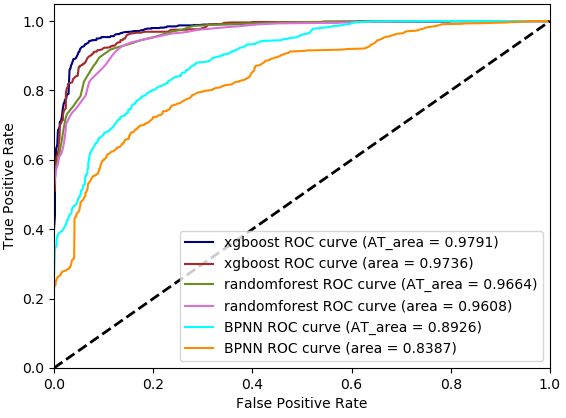
This paper uses the output of the XGBoost model as one Figure.1 ROC curve of level I diagnostic layer
of the evidences, and its basic probability value is
calculated as follows:
& N1 #
m( Ri ) y ( Ri ) / $
$
y ( Ri ) En !
!
(10)
% i 1 "
y ( Ri ) is the output probability value of the XGBoost
model, E n is the error,
1
En (t j y j ) 2 (11)
2
t j is the actual one hot label, y j is the output probability
value of the XGBoost model, Ri ( i 1ˈ 2ˈ
ˈN1 )is the
fault category; N1 is the total number of fault categories. Figure.2 ROC curve of level II diagnostic layer
Other evidence uses statistical methods to determine its Take the I and II diagnostic models as an example, the
basic probability value. ROC[10] curves are shown in Figures 1 and 2 respectively.
The first level only uses the XGBoost model. It can be
seen from Figure 1 that after arctangent processing, the
3.5 The algorithm flow of XGBoost
AUC area of the level I diagnostic model has increased
1) Divide 1014 inspection data into 811 training set and by 0.0209 to 0.9764. For the same reason, Figure 2 shows
203 test set according to 4:1, and use the reduced that the AUC area of the three models XBGboost, Rand-
attributes as input to complete the training of the omForest, and BPNN after arctangent processing increas-
XGBoost model, and use 203 test set data for prediction ed by 0.0217 on average, and the AUC area stratification
to verify the performance of the XGBoost model . occurred: the AUC area of XBGboost is larger than
2) Input the data to be diagnosed into the trained RandomForest, and the AUC area of RandomForest is
XGBoost model according to the reduced attributes to larger than BPNN. It shows that through arctangent
obtain the output probability value. transformation, the input data is mapped to [0, ' /2], and
3E3S Web of Conferences 243, 01002 (2021) https://doi.org/10.1051/e3sconf/202124301002
ICPEME 2021
then normalized processing can effectively solve the of accuracy rate, it can be obtained that the predictive
long-tailed[11] distribution problem of DGA data, so that ability of XGBoost diagnostic models at all levels is the
the model can better express the nonlinear relationship best after being reduced by the neighborhood rough set
between input and output . theory.
Table 3. Time-consuming diagnosis of different input
4.2 Comparison of accuracy after feature reduct- characteristic parameters at all levels(s).
ion
Diagnostic Layer S1 S2 S3 S4
Supposing five characteristic gases are input characterist- XGBoost1 0.0279 0.1165 0.0654 0.0569
ic parameters S1 ,and the ratio of 9 characteristic gases of XGBoost2 0.0863 0.0469 0.1178 0.1374
the non-code ratio method is input characteristic paramet- XGBoost3 0.0754 0.0359 0.0517 0.0489
XGBoost4 0.0614 0.0437 0.0569 0.0455
ers S 2 , five characteristic gases and the ratios of 16 char- XGBoost5 0.0864 0.0325 0.0629 0.0588
acteristic gases are input characteristic parameters S3 , Calculate the average time for each of the five models
The input feature parameter after reducing S3 by the of the four characteristic parameters. The longest average
time is the five characteristic gases and the ratios of the
neighborhood rough set theory is S 4 , Input the above four
16 characteristic gases ( S3 ), the value is 0.07094s. The
characteristic parameters into the XGBoost graded diagn-
shortest average time is non-code ratio method( S2 ),
osis model, and get Tables 2 and 3.
which has a value of 0.0551s, and the average time it
Table 2. Diagnosis accuracy rates of different input feature takes to input the features to all levels of models after
parameters at all levels(%). attribute reduction( S4 ) is 0.0695s, which is shorter than
Diagnostic Layer S1 S2 S3 S4 S3 and meets actual requirements.
XGBoost1 90.14 90.96 93.86 95.40
XGBoost2 87.95 89.96 90.99 92.62
XGBoost3 86.67 87.53 91.38 92.02
4.3 Comparison of different diagnostic methods
XGBoost4 85.04 85.41 89.29 91.36
XGBoost5 86.91 90.34 89.34 90.95 Taking the hierarchical diagnosis proposed in this
Observing Table 2, we can see that the diagnostic paper as a model, using the reduced feature parameters in
accuracy of level I of the four input feature parameters is as the input of BPNN, RandomForest and XGBoost,
the highest compared to level II and III, all of which are respectively, the accuracy comparison histogram of each
above 90%, and the highest is 95.40%. This is because classifier under different methods is obtained. In the
the I-level XGBoost model can easily grasp the Figure 3, N-F means normal and fault, C-H-M means
difference between the characteristics of normal and fault discharge, overheating and complex faults. For the
data through learning. The accuracy of the four feature description of other fault types, see section 3.1 .
quantities as the input of the II and III models has
decreased, indicating that when the fault type needs to be
specifically subdivided, the generalization ability of the
model is more demanding. In level II diagnosis, due to
the large sample size, the generalization ability of the
model is effectively improved through learning, so the
accuracy rate is high. The average accuracy of level II is
90.38%, and the highest is 92.62% for S 4 .
Since the five characteristic gases are directly used to
distinguish fault types from DGA data, they contain more
redundant information, so the level III diagnosis accuracy
of the five characteristic gases is low, with an average
accuracy rate of only 86.21%. The non-code ratio method Figure.3 Comparison of accuracy rates between various
is used as the input feature parameter. Since the ratio classifiers
selection is only 9 kinds, it is not comprehensive and Figure 3 shows that the XGBoost model has the high-
detailed, and it is easy to cause uncertainty in reasoning. est accuracy rate compared to BPNN and RandomForest
Therefore, the average accuracy rate of the third level of at the same level of diagnosis, which is 0.06046 higher
the non-code ratio method is only 87.76%. than BPNN on average and 0.02774 higher than Random-
When the five characteristic gases and the ratios of 16 Forest on average. From the perspective of the AUC area
characteristic gases are used as input parameters, because under the ROC curve, the XGBoost model has the largest
the included fault characteristic information data is AUC area with a value of 0.9791, which is 0.0865 and
relatively complete and accurate, the average accuracy 0.0127 higher than BPNN and RandomForest, respective-
rate of level III reaches 90%. When the feature ly. It can be seen that the XGBoost model proposed in th-
parameters after attribute reduction are used as input, the is paper has the best effect among the several classifiers.
diagnostic model of each level has selected features, so At the same time, it can be seen from Figure 3 that when
the accuracy of each level is the highest, and the average the fault types are subdivided level by level, the accuracy
accuracy of level III is 91.44%. Through the comparison rate decreases. This is due to the limited sample size,
4E3S Web of Conferences 243, 01002 (2021) https://doi.org/10.1051/e3sconf/202124301002
ICPEME 2021
unbalanced data, and the generalization ability of the Through the level I decision fusion, the conclusion
model is limited. can be drawn: the operating condition is a fault, the unce-
The sample labels are set to the nine fault types rtainty is 9.5 (10-7 , the confidence interval is (0.9974,
proposed by the non-code ratio method, and the nine 0.99740095), and the reliability of the level I model for
characteristic gas ratios proposed by the non-code ratio diagnosing the operating condition as fault F is improved.
method are used as the input of BPNN and RandomFore- Further analysis, there are three possible fault types:
st, which do not use a graded model, and compared with discharge (C), overheat (H), and complex (M). input the
the prediction accuracy of the XGBoost graded diagnosis reduced feature parameters into the class II XGBoost2
model proposed in this paper. Table 4 can be obtained. model, the actual output of the class II model is [0.9389,
Table 4. Fault diagnosis accuracy rate of different methods(%). 0.0359, 0.0252], and the expected output is [1, 0, 0].
According to equations (10) and (11), the basic
Diagnosis Non-code
BPNN
Random XGBoost probability distribution of evidence source e3 is calculated
Method Ratio Forest Graded
Accuracy 88.46 90.14 91.91 93.01
as [0.9363, 0.0358, 0.0251], and the basic probability
distribution of another evidence source e4 is calculated as
Table 4 indicates that due to the limited fault feature
information contained in the non-code ratio method, the [0.3829, 0.3160, 0.2009] based on the analysis of failure
accuracy rate is only 88.46%, BPNN is easy to fall into statistical data, then available Table 8:
the local optimum, and the accuracy rate is only 90.14%. Table 8. Probability distribution of level II diagnostic model.
XGBoost is more suitable for processing data with a few
features than RandomForest, and considering the second Evidence
Basic Probability
Uncertainty
derivative, adding regular term coefficients to the loss C H M
function, and pre-pruning the decision tree, its accuracy is e3 0.9363 0.0358 0.0251 0.0028
1.1% higher than RandomForest, reaching 93.01%. e4 0.3829 0.3160 0.2009 0.1002
Using formulas (5)—(8) in the D-S evidence theory
5 Case of study for fusion, the conflict factor K can be obtained as 0.4775.
The confidence and likelihood of various failure types are
Taking the DGA data in Table 5 as an example, the fault shown in Table 9. The conclusion can be drawn from the
type is high-energy discharge. This article uses D-S second-level decision: the fault type is discharge, the
evidence theory to conduct information fusion[12] analysis. uncertainty is 0.0005, and the confidence interval is
(0.9495, 0.95), and the reliability of the second-level
Table 5. Transformer DGA data(ul/L).
model for diagnosing the fault type as discharge is
H2 CH 4 C2 H 6 C2 H 4 C2 H2 improved.
164.56 36.65 9.88 85.97 193.83 Table 9. Confidence and likelihood of various failure types
Input the reduced characteristic parameters into the
hierarchical XGBoost diagnosis model in turn. The actual Fault Type Bel Pl
output of the I-level XGBoost1 model is [0.0221, 0.9779], C 0.9495 0.9500
and the expected output is [0, 1]. According to equations H 0.0320 0.0325
(10) and (11), the basic probability distribution of M 0.0170 0.0175
evidence source e1 is [0.0220, 0.9774]. The analysis of There are three possibilities for this level of diagnosis
from the diagnosis result of the upper level as discharge:
transformer fault statistics data shows that the basic
low-energy discharge ( D1 ), high-energy discharge ( D 2 )
probability distribution of another source of evidence e2
and partial discharge (PD), input the reduced features into
is [0.0986,0.9000], then Table 6 can be obtained:
the III-level XGBoost5 model, the actual output is
Table 6. Probability distribution of level I diagnostic model. [0.0281, 0.9507, 0.0212], and the expected output is [ 0, 1,
0]. According to formulas (10) and (11), the basic
Evidence
Basic Probability
Uncertainty probability distribution of evidence e5 is calculated as
N F
e1 [0.0280, 0.949, 0.0211], and the basic probability
0.0220 0.9774 0.0006
distribution of evidence e6 as which the non-code ratio
e2 0.0986 0.9000 0.0014
method act is [0.27, 0.51, 0.21], then Table 10 :
According to formulas(5)—(8), carry out evidence
fusion and calculate the conflict factor K to be 0.8838. Table 10. Probability distribution of level III diagnostic model.
The confidence and likelihood of various operating
Basic Probability
conditions are shown in Table 7: Evidence Uncertainty
D1 D2 PD
Table 7. Confidence and likelihood of various operating e5 0.0280 0.9490 0.0211 0.0019
conditions.
e6 0.2700 0.5100 0.2100 0.0100
Fault Type Bel Pl In the same way, the conflict factor K is 0.5079, and
N 0.0025 0.00250095 the confidence and likelihood of various failure types are
F 0.9974 0.99740095 shown in Table 11:
5E3S Web of Conferences 243, 01002 (2021) https://doi.org/10.1051/e3sconf/202124301002
ICPEME 2021
Table 11. Confidence and likelihood of various failure types diagnosis with unbalanced samples based on neighb-
orhood component analysis and k-nearest neighbors,
Fault Type Bel Pl ” (2020)
D1 0.0164 0.016437 2. Wu Zhenyu, Zhou Lijun, Zhou Xiangyu, Lin Tong,
D2
Guo Lei, Liu Hongwen and Jiang Junfei, “Research
0.9735 0.973537
on fault diagnosis method of transformer winding
PD 0.0099 0.009937 based on oscillatory wave,” Proceedings of the CSEE,
The conclusion can be drawn from the third-level vol. 40, pp. 348–357, (2020)
decision: the fault type is high-energy discharge, the 3. Liu Hang, Wang Youyuan, Chen Weigen, Liu Lifeng,
and Zhang Jianguang, “Fault detection for power
uncertainty is 3.7 (10-5 , the confidence interval is (0.9735,
transformer based on unsupervised concept drift rec-
0.973537), and the reliability of the third-level model in ognition and dynamic graph embedding,” Proceedin-
diagnosing the fault type as high-energy discharge is gs of the CSEE, vol. 40, pp. 4358–4370, (2020)
improved. 4. Li Gang, Yu Changhai, Fan Hui, Liu Yunpeng and
Song Yu, “Deep fault diagnosis of power transform-
6 Conclusion er based on multilevel decision fusion model,” Elect-
ric Power Automation Equipment, vol. 37, pp.138–
144, (2017)
Based on the XGBoost model, this paper uses the neighb- 5. Wu Xiaoxin, He Yigang, Duan Jiajun, Zhang Hui, Z-
orhood rough set theory to reduce its input, and uses its eng Zhaorong, “Bi-LSTM-based transformer fault d-
output as one of the evidence sources to employ D-S iagnosis method based on DGA considering comple-
evidence theory for information fusion, and establish the x correlation characteristics of time sequence”, Elect-
XGBoost graded diagnosis model, which is compared ric Power Automation Equipment, vol. 40, pp. 184–
with the non-code ratio method, BPNN and RandomFore- 190,(2020)
st, the prediction accuracy of the transformer graded 6. Yin Shi, Hou Guolian, Hu Xiaodong, Zhou Jiwei, G-
diagnosis model proposed in this paper is higher than ong Linjuan, “Fault warning and identification of fr-
2.7% on average, and the average time from training ont bearing of wind turbine generator,” Chinese Jour-
model to prediction is less than 0.07 s. In the analysis of nal of Scientific Instrument, vol. 41, pp. 242–251,
the examples, the D-S evidence theory was used to verify (2020)
the efficiency and reliability of the diagnosis model at all 7. Pang Mengyang, Suo Zhongying, Zheng Wanze, Xu
levels proposed in this paper. After summarizing, the YuHeng, Bao Zhuangzhuang and Huang Lin, “Small
following conclusions are drawn: sample fault diagnosis of aeroengine based on RS-
CART decision tree,” Journal of Aerospace Power,
1) By preprocessing the data with arctangent tran-
vol. 35, pp. 1559–1568, (2020)
sformation, and then normalizing, the AUC area of the
8. Ma Suliang, Jia Bowen, Wu Jianwen, Yuan Yang,Ji-
model can be increased, and the long-tailed distribution
ang Yuan and Li Weixin, “Multi-vibration informati-
problem of DGA data can be solved. on fusion for detection of HVCB faults using CART
2) The feature attribute reduction using the neighbor- and D-S evidence theory,” (2020)
hood rough set theory can retain the features that have a 9. Gao Rong, Kou Peng, Liang Deliang, Liu Yibin, Wu
greater contribution to distinguishing fault types and rem- Zihao, “Robust model predictive control for the volt-
ove redundant features, which can improve the prediction age regulation in active distribution networks with
accuracy and shorten the model training time . Hybrid distribution transformers,” Proceedings of the
3) Through the use of D-S evidence fusion theory, the CSEE, vol. 40, pp. 2081–2090, (2020)
ambiguity is resolved. In the future, more sufficient data 10. Fawcett Tom, “An introduction to ROC analysis,” P-
will be used to establish the XGBoost hierarchical attern Recognition Letter, vol.27, pp.861–874, (2006)
diagnosis model, which can solve the problem of data 11. Chu P, Bian X, Liu S and Ling H, “Feature space
imbalance, so that all levels of models have a high augmentation for long-tailed data,” (2020)
diagnostic accuracy rate, and there will be no decline. 12. Li Yonggang, Wang Luo, Li Junqing and Ma Mingh-
an, “Identification of inter-turn short-circuit fault in
rotor windings of synchronous generator based on
References multi-source information fusion,” Automation of El-
ectric Power Systems, vol.43,pp.162–167,191,(2019)
1. Li Yaxin, Hou Huijuan, Zhang Lijing, Xu Mingkai,
Sheng Gehao, and Jiang Xiuchen, “Transformer fault
6You can also read


