Analysis of spatial patterns and driving factors of provincial tourism demand in China
←
→
Page content transcription
If your browser does not render page correctly, please read the page content below
www.nature.com/scientificreports
OPEN Analysis of spatial patterns
and driving factors of provincial
tourism demand in China
Xuankai Ma1,2,3, Zhaoping Yang2* & Jianghua Zheng1
Modeling and forecasting tourism demand across destinations has become a priority in tourism
research. Most tourism demand studies rely on annual statistics with small sample sizes and lack
research on spatial heterogeneity and drivers of tourism demand. This study proposes a new
framework for measuring inter-provincial tourism demand’s spatiotemporal distribution using search
engine indices based on a geographic perspective. A combination of spatial autocorrelation and
Geodetector is utilized to recognize the spatiotemporal distribution patterns of tourism demand in
2011 and 2018 in 31 provinces of mainland China and detect its driving mechanisms. The results reveal
that the spatial distribution of tourism demand manifests a vital stratification phenomenon with
significant spatial aggregation in the southwest and northeast of China. Traffic conditions, social-
economic development level, and physical conditions compose a constant and robust interaction
network, which dominates the spatial distribution of tourism demand in different development stages
through different interactions.
Tourism is an essential driver of world economic development. The world was affected by the COVID-19 out-
break in 2019, and according to a report by the World Tourism Organization1, the world’s top ten consumer
countries showed continued growth in tourism consumption against the backdrop of a global economic slow-
down. According to the Ministry of Culture and Tourism of the People’s Republic of China (https://www.mct.
gov.cn/), China’s 2020 annual domestic tourism numbered 2.879 billion trips, down 52.1% from a year earlier.
The first quarter of 2021 saw 11.872700 billion domestic trips organized by national travel agencies, increasing
138.50% year-on-year. As the contribution of tourism to the regional economy is improving more and more
significantly, the study of tourism demand has become a popular research topic2. Many scholars have carried out
tourism demand forecasting through qualitative analysis, time series models, econometric models with artificial
intelligence, and the accuracy of forecasting has gradually improved. However, tourism and tourists are closely
correlated in terms of spatial mobility, and if spatial effects are ignored, a model estimation can be biased and
produce misleading coefficient estimates3–5. Deng and Athanasopoulos were the first to incorporate spatiotem-
poral dynamics into an Australian domestic tourism demand model s tudy6, and Yang and Zhang showed that
spatiotemporal models have a significantly enhanced effect on the performance of tourism demand forecasting
between domestic provinces in C hina7. Liu et al. noted that demographic factors, climate, key transportation
modes, economic level, and other aspects of tourism demand were not i nvestigated8. Therefore, it is imperative
to understand the spatiotemporal patterns and driving mechanisms of tourism demand.
From the tourism supply side, the geographical and spatial clustering of tourism-related services produces
spatial dependence and scale effects at the macro level, thus providing tourists with more acceptable prices and
convenient services to achieve regional tourism growth. From the tourism demand side, tourists from the same
region have more similar social psychology and tourism demand9, their tourism demand patterns are similar in
terms of spatial preferences, and travel patterns show a more consistent cyclicality in time. Domestic tourism is
an undisputed driver of economic development and poverty alleviation in less developed regions than interna-
tional tourism10. Pompili et al. argued that choosing the provincial level as the geographic unit to study tourism
flows yields more valuable results11. The results of the detection of spatial effects within a region can provide a
scientific and empirical reference to local governments, tourism planners and administrative units regarding
resource allocation and infrastructure development.
Several studies have explored the factors affecting tourism demand. For example, Priego et al. explored the
impact of climate change on domestic tourism flows in S pain12. Massidda and Etzo studied the contribution of
1
College of Resource and Environment Sciences, Xinjiang University, Ürümqi 830046, China. 2Xinjiang Institute
of Ecology and Geography, Chinese Academy of Sciences, No.818, Beijing South Road, Ürümqi 830011, Xinjiang,
China. 3University of Chinese Academy of Sciences, Beijing 100049, China. *email: yangzp@ms.xjb.ac.cn
Scientific Reports | (2022) 12:2260 | https://doi.org/10.1038/s41598-022-04895-8 1
Vol.:(0123456789)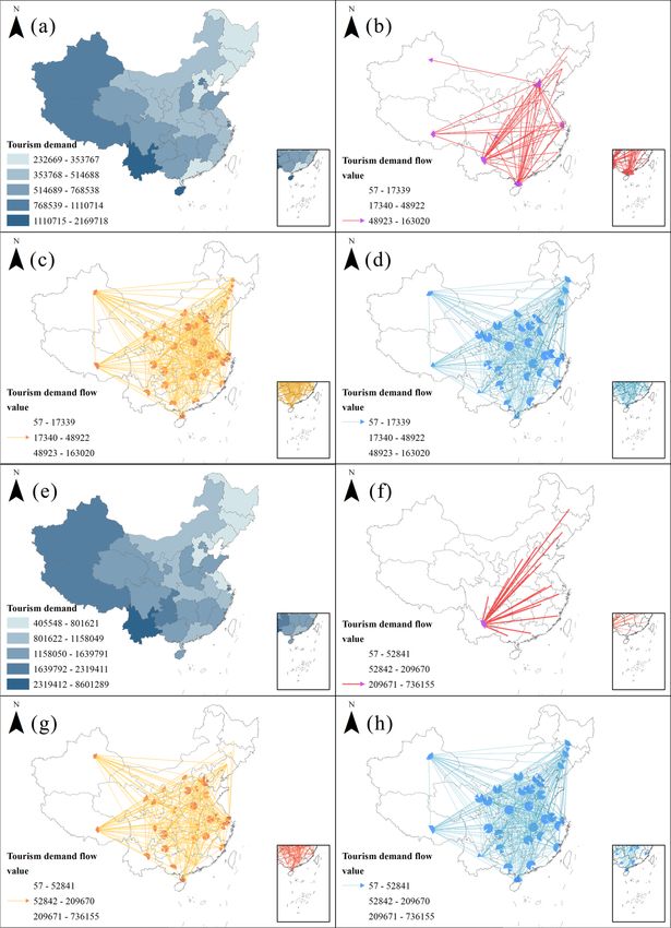
www.nature.com/scientificreports/
road infrastructure to tourism demand in domestic tourism in Italy9. Priego et al. emphasize the importance of
meteorological factors on domestic travel destinations in S pain12. Technological innovation13 and knowledge
spillovers14 cannot be ignored in driving tourism productivity and making tourism demand grow. Alvarez‐Diaz
et al.15, Marrocu and Paci16, Massidda and E
tzo9 confirmed that the size of the population is also one of the drivers
of tourism demand. Despite the large number of studies exploring the factors affecting tourism demand, most
researchers have focused more on the impact of single aspects of socio-economic or natural factors on tourism
demand, and there are no studies based on a geographic perspective that integrate the various dominant factors
into a comprehensive mechanism of impact on tourism demand.
We found from the early literature that the number of tourists and tourism income served as the main proxies
for tourism demand modeling. With the development of the Internet, some r esearchers8,17 found that tourists’
search engines for tourism information retrieval are the starting point and an essential part of tourism decision
and travel. Li et al. summarized relevant 2012–2019 in their latest r eview18. We know about search engine data
primarily based on empirical studies investigating the eximious contribution to tourism demand observation
and forecasting. With Google Trends being widely used for tourism demand forecasting at multiple spatial
scales worldwide19, Baidu Index performs even better in the Greater China region20. Song et al. demonstrated
that Internet data has a significant driving effect on tourism demand research, with search engine data being the
most common Internet data source used by r esearchers19. It is now well established from various literature that
analytical methods have been implemented to address the single driving mechanisms of tourism demand. In their
paper, Marrocu and Paci indicated that the application of spatial autoregressive models gave the spatial depend-
ence patterns of tourism flows access to be effectively presented16. Yang and Fik investigated tourism growth
change in 342 cities in China using spatial growth regression m odels21. Deng et al. used a spatial econometric
analysis framework to analyze the impact of air pollution on inbound tourism in China22. In general, tourism
demand is not affected by any individual factor, and the interactions among the factors affect the distribution of
tourism demand. Therefore, it is crucial to detect the interrelated effects of tourism demand drivers. However,
most existing studies ignore the interaction among the drivers of tourism demand. In addition, most existing
models used in the literature make assumptions about the data and fail to reveal the interaction among the factors.
To fill these gaps, this study aims to address the spatial heterogeneity and drivers of tourism demand by
using 678,900 Origin–Destination flows (OD flows) of tourism demand data from 31 Chinese provinces at the
years 2011 and 2018, which helps gain insight into the spatial heterogeneity of tourism demand exhibited in
the period of rapid economic development. Second, to our knowledge, this might be the first attempt to present
a theoretical framework for a multi-factor driving mechanism of tourism demand, which incorporates social-
economic development, population size, urban ecological conditions, tourism resources, physical conditions,
traffic conditions, and technological innovation. Third, from the perspective of spatially stratified heterogeneity,
this study taps the influence of the main driving factors and the interaction between different potential factors
on the spatial heterogeneity of tourism demand. In addition, the study of tourism demand should not only focus
on the influence of local economic activities and the natural environment but also the influence of inter-regional
spatial correlation. Therefore, this study uses spatial autocorrelation and geographic detector models to analyze
the spatial variation of tourism demand and its drivers at the provincial level.
The rest of the study is organized as follows: “Materials and methodology” section provides an overview of
the proxies affecting tourism demand and the data and methods used in this paper. “Results” section analyzes
the drivers and spatial characteristics of tourism demand. Finally, “Discussion” and “Conclusions” sections are
the discussion and conclusion of the findings, respectively.
Materials and methodology
Study areas. After the world economic crisis in 2008, China started its economic recovery in 2011, followed
by an average annual growth of 9.48% in GDP and 14.99% in total domestic tourism consumption until 2018
(Fig. 1b,c). This paper investigates the factors driving the changes in the spatial distribution of tourism demand
at a provincial level in China in 2011 and 2018 to provide a basis for planning decision-makers in developing
countries and regions. This study regarded the provinces as the primary geographical unit, and 31 administra-
tive provinces in mainland China were selected as the study area. Due to the unavailability of data, Hong Kong,
Macao, and Taiwan are not included in the study area (Fig. 1).
Dominant factors and proxy variables of tourism demand. From a systemic perspective, the under-
lying driving mechanism of tourism demand is constituted by the tourist travel intention of the source and the
destination’s attractiveness. It is influenced by the resistance of temporal distance, spatial distance, and social
distance23–25. Natural conditions and human factors determine tourism demand (Fig. 2). In this study, social-
economic development (Z1), population (Z2), urban ecology (Z3), tourism resources (Z4), physical conditions
(Z5), traffic conditions (Z6), and technology innovation (Z7) are used as factors that directly affect tourism
demand. Considering the availability of data, GDP per capita, value-added of tertiary industry, and the average
wage of employees is used to characterize the level of socio-economic development. The total population and
nighttime light index measure the population scale. Urban ecological condition is indicated by Urban park green
area. Museums and A-class scenic spot index represent the richness of tourism resources. The physical environ-
mental conditions consist of altitude, average daily hours of sunshine, average daily temperature, green space
coverage index. Transportation conditions are reflected by the urban road area, highway mileage, and railroad
mileage. The number of enterprises in the high-tech industry represents the region’s scientific and technological
innovation capability. The search intensity of the Baidu index was employed to quantify tourism demand.
Scientific Reports | (2022) 12:2260 | https://doi.org/10.1038/s41598-022-04895-8 2
Vol:.(1234567890)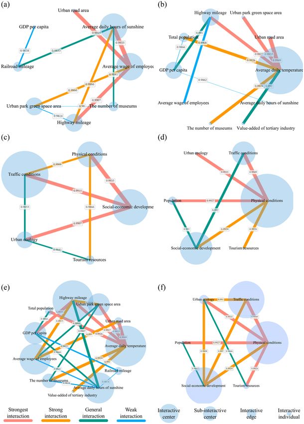
www.nature.com/scientificreports/
Figure 1. An overview map of the study area: (a) 31 provinces in mainland China; (b) economic conditions in
the study area from 2011–2018; (c) tourism in the study area from 2011 to 2018. Data on China’s economy are
from the National Bureau of Statistics of China (http://www.stats.gov.cn/) and the Chinese Academy of Social
Sciences (http://english.cssn.cn/). Standard map services are provided by the Ministry of Natural Resources of
China (http://bzdt.ch.mnr.gov.cn/), GS (2020)4619.
Figure 2. Determinants and their geographical proxy variables concerning the spatial distribution of tourism
demand.
Data. Tourism demand of inter‑province. Search engine big data are one of the data sources that can accu-
rately quantify tourism demand. Search engines collect records of Internet users retrieving information on the
Internet to form search engine indices with high timeliness. Baidu index (https://index.baidu.com/) has better
accuracy in the Greater China region for measuring tourism demand, and keywords query it. The keyword
database consisted of the combinations of destination provinces name + "tourism". The Baidu index of each
keyword could be decomposed according to the region and time, to obtain the daily search intensity of internet
users in province A for tourism information in province B. We constructed an origin–destination (OD) spati-
otemporal matrix in 2011 and 2018, which contains the intensity of travel information retrieved by residents
Scientific Reports | (2022) 12:2260 | https://doi.org/10.1038/s41598-022-04895-8 3
Vol.:(0123456789)
www.nature.com/scientificreports/
Figure 3. Correlation matrix of tourism demand between provinces: Based on the daily Baidu indexes
accumulated throughout the year in (a) 2011; (b) 2018. The Y-axis is the origin, and the X-axis is the
abbreviation that replaces the destination, the name of each province. The color of each grid represents the total
annual amount of tourism demand from the source province to the destination province. The grid color From
lighter to darker represents the strength of tourism demand flow.
of one province on the Internet for another province for each day. The correlation matrix of tourism demand
among provinces visualized in Fig. 3 was obtained by summing up the daily tourism demand flows by year and
accumulated in terms of destination provinces to obtain the tourism retrieval index of each province for a year.
It characterized the total tourism demand of that province. Additionally, the annual Baidu Index of province-A
Internet users query for tourism information about province-B is defined as a tourism demand flow for this OD.
Indicators for influencing factors. We collected statistical panel data released in 2012 and 2019 from the China
City Statistical Yearbook (http://www.stats.gov.cn/tjsj/tjcbw/), including official statistics on the economic devel-
opment level, population, urban ecological conditions, transportation conditions, and science and technology
innovation. A-class tourism resources lists were extracted from the summary of government documents pub-
lished on each local government website, and the tourism resources were numerically mapped according to A-1,
AA-2, AAA-3, AAAA-4, and AAAA-5 remapping. The tourism resource addresses were geocoded into spatial
point data, and kriging interpolation was implemented for spatial interpolation to generate the A-class tourism
resources index raster. In addition, we used remote sensing data as a geographic proxy variable for physical
conditions and population distribution. The NPP-VIIRS-like NTL Data from Harvard Dataverse (https://libra
ry.harvard.edu/services-tools/harvard-dataverse/), which represents the intensity of human activity at night, the
elevation data is from the Resource and Environmental Science Data Center of the Chinese Academy of Sciences
(https://www.resdc.cn/), the climate data is from the National Meteorological Science Data Center of China
(http://data.cma.cn/), and the green space coverage index is from the USGS (https://www.usgs.gov/). All proxy
variables were free of being counted according to provincial administrative boundaries, and the raw data were in
a GeoDetector model where sampling points would capture the values of different variables.
Methodology. Exploratory spatial data analysis. Exploratory spatial data analysis is a series of spatial data
statistical analyses applied to describe and visualize the spatial and temporal distribution patterns of tourism
demand. Global spatial a utocorrelation26 is adopted to determine whether the spatial distribution pattern of
tourism demand is clustered, dispersed, or random27. The local spatial autocorrelation28 is practiced in identify-
ing areas where spatial clustering and outliers occur to explore their spatial effects29. Considering the spatial data
of provinces are polygons and checked by topology, Queen contiguity is utilized to indicate the spatial weight
matrix between provinces30.
Spatial stratification heterogeneity analysis. GeoDetector is an advanced spatial statistical analysis model used
to study factors’ impact on diseases at a specific geographical area early31. Furthermore, it gradually developed
into various research fields with spatial characteristics, such as ecological security, food production, urban land
use, carbon emissions. It is a hypothesis that if the independent variable directly influences the dependent varia-
ble in space, then the spatial distribution of the dependent variable should converge with the spatial distribution
of the independent variable32. The model detects the similarity of two variables in spatial distribution patterns
from the perspective of spatially stratified heterogeneity33.
In this paper, GeoDetector was adopted to analyze the factors affecting the spatial distribution of tourism
demand in 31 provinces of China (Fig. 4). Factor detection, ecological detection, and interactive detection
submodules were applied to quantify their spatial heterogeneity and interactions between factors on the spatial
distribution of tourism demand. The Q statistic measured and explained the influence of the independent vari-
able X on the dependent variable Y on spatial heterogeneity. The expressions are as follows.
Scientific Reports | (2022) 12:2260 | https://doi.org/10.1038/s41598-022-04895-8 4
Vol:.(1234567890)
www.nature.com/scientificreports/
Figure 4. Principle of geodetector.
M 2
j=1 Nj σj
Q =1− (1)
Nσ 2
where: Q-statistic is a measure of the explanatory power of the influence of factor X on tourism demand Y; M
represents the number of strata (subdivisions); N represents the number of provincial geographical units in the
study area; Nj represents the number of provinces in subdivision j ; σ 2 and σj2 indicate the variance of tourism
demand in the whole study area and the variance of tourism demand in each subdivision, respectively. The greater
the value of Q, the stronger the influence of factor X on tourism demand Y.
Stratification of geographic proxy variables has a significant impact on the accuracy of factor detection. The
optimization algorithm for stratifying geographic proxy variables parameters proposed by Song et al. offered
optimizing spatial d iscretization34. The optimization algorithm assumes that each variable is stratified using dif-
ferent unsupervised discretization methods to form different stratification schemes. If one alternative scheme
obtains an enormous Q-statistic based on factor detection calculations, this stratification scheme captures the
most significant driving force between that variable and the observed variables.
The study area was spaced at 50 km intervals, and 3795 sampling points were generated to sample 16 con-
tinuous-type variables. Quantile method, natural break method, geometric break method, standard deviation
break method, and equivalence breakpoint method were used as statistical stratification methods with intervals
of 3–6, and the Q-statistic of proxy variables and observations under different stratification schemes were probed.
Finally, the scheme with the enormous Q-statistic was selected as the stratification and interval parameters for
this proxy variable.
Results
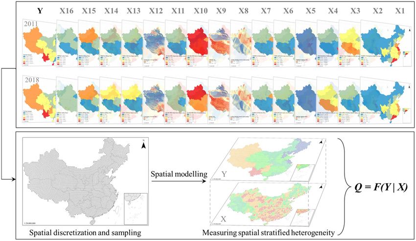
Spatial patterns of tourism demand in provinces. Spatial distribution. Figure 5 illustrates the spatial
distribution of tourism demand and flows between provinces in 2011 and 2018. In 2011, tourism demand was
mainly distributed in China’s first-tier cities with Beijing and Shanghai and the border provinces from southwest
to northwest, with Hainan, Yunnan, Tibet, and Xinjiang being the main tourism demand destinations 35.33%
of tourism demand in the study area. In 2018, tourism demand showed a trend of migration to first-tier cities,
with Yunnan, Tibet, Shanghai, Chongqing, and Guizhou accounting for 36.46% of the total tourism demand.
From the spatial perspective of tourism flow, there are 930 tourism flows between provinces with a minimum
Euclidean distance of 115 km, a maximum of 3600 km, and a median of 1286 km. Long-distance travel35 is a
characteristic of tourism between domestic provinces. In 2011 the tourists’ origins were concentrated in eastern
China, and there were two clusters of high-intensity tourism flows distributed from Beijing and the ring-Beijing
area to Yunnan and Hainan; this phenomenon altered significantly in 2018, with high-intensity tourism flows
concentrated on one cluster of tourism flows from eastern China to Yunnan Province. Medium-intensity tour-
ism flows presented a complex network with a stochastic pattern in 2011; in 2018, the complexity of the tourism
network decreased, with steady clusters of tourism flows originating from the eastern provinces to Xinjiang and
Scientific Reports | (2022) 12:2260 | https://doi.org/10.1038/s41598-022-04895-8 5
Vol.:(0123456789)
www.nature.com/scientificreports/

                                           Figure 5.  Spatial distribution of tourism demand and tourism demand flow: (a) tourism demand in 2011, and
                                           (e) is in 2018; (b–d) are the inter-provincial directional tourism demand flows in 2011, which are high-intensity
                                           flow, medium intensity flow, and low-intensity flow respectively, and (f–h) is in 2018.

                                           Tibet, while the northeastern region became a complete exporter of tourists. Comparing the low-intensity tour-
                                           ism flows in 2011 and 2018, it can be attended that the overall origin and destination were practically completely

          Scientific Reports |   (2022) 12:2260 |               https://doi.org/10.1038/s41598-022-04895-8                                                 6

Vol:.(1234567890)
www.nature.com/scientificreports/

                                 Figure 6.  Spatial distribution of the ratio of tourism demand in 2018 to 2011.

                                 connected, i.e., there were tourism flows from both border provinces and the central region. The central provinces
                                 also energetically export tourists to the peripheral provinces, diverting the overall tourism flow network to a
                                 more luxuriant state. In summary, we can catch that the domestic tourism network in China during the period
                                 of rapid economic development showed a remarkable complex pattern, with the origins of tourists consolidated
                                 in the densely populated and economically developed areas in the east and the destinations distributed in the
                                 first-tier cities, and remote areas in the central and western regions.
                                     From 2011 to 2018, the northeastern provinces, Beijing-Tianjin-Hebei region (Beijing, Tianjin, Hebei), Yang-
                                 tze River Delta region (Shanghai, Jiangsu, Zhejiang, Anhui), and Pearl River Delta region (Guangzhou) are stable
                                 tourist sources; the average value of tourism demand in each province rose from 642,515 to 1,529,387, an increase
                                 of 2.38 times (Fig. 6). Yunnan and Guizhou in the southwest and Gansu in the west grew at a much higher rate
                                 than the national average; Heilongjiang, Jilin, and Liaoning in the northeast grew at a much lower rate than the
                                 average; and Hainan in the south became the only province in the country where tourism demand decreased.

                                 Spatial dependency. The spatial distribution pattern of tourism demand shifted from medium to high cluster-
                                 ing in 2011 and 2018, and the positive Moran’s I revealed the existence of high-value to high-value clustering
                                 or low-value to low-value clustering of tourism demand in the study area, and the spatial pattern and spatial
                                 dependence of tourism demand with evident clustering. The z-score increased by 177.58% during this period,
                                 and the p-value decreased by 88.96%. The probability of rejecting the null hypothesis increased from 90 to 95%.
                                 Thus, the spatial clustering trend of tourism demand strengthened.
                                     The global Moran’s I identified the overall spatial dependence of tourism demand in each province within the
                                 study area, and Local spatial autocorrelation analysis was applied to uncover the local spatial association patterns.
                                 As can be seen from Fig. 7, significant stratification of tourism demand in 2011 and 2018 on a local spatial basis
                                 in China (absolute value of Z-score > 2.56, p-value < 0.01), consisting mainly of high-high value clusters (H–H)
                                 and low-low value clusters (L-L). In 2011, the H-H cluster was in Yunnan Province in southwestern China, the
                                 high values surrounded by low values cluster (H-L) appeared in Beijing, and the L-L cluster was in Heilongjiang
                                 Province in northeastern China. In 2018, the H-H cluster was still in Yunnan province, and the L-L clusters
                                 were distributed in Heilongjiang, Jilin, and Liaoning province, covering the whole northeastern region. From
                                 the perspective of spatial and temporal distribution, tourism demand formed a growth pole in southwestern
                                 China centered on Yunnan from 2011 to 2018, and tourism demand in Guizhou, adjacent to Yunnan, grew
                                 significantly and showed a spatial diffusion effect the region (Fig. 7). While in northeast China, the number of
                                 L-L clusters increased, and the provincial growth rate of tourism demand in low-value agglomeration was much
                                 lower than the national average during the study period. The existence of the H-L cluster in Beijing in 2011 and
                                 the disappearance of this cluster in 2018 indicated that Beijing had strong competitiveness in the region in the
                                 early stage, and the weakening polarization effect and the increasing diffusion effect diminished in the later stage
                                 when tourism demand was gradually distributed in a balanced manner in the Beijing-ring region. It suggested
                                 that tourism demand was more stable in China spatially in high-value clustering, and low-value clustering had
                                 increased, forming an increasingly stable high-value area in the southwest and low-value area in the northeast.
                                 Therefore, tourism demand in one province largely influences tourism demand in the adjacent provinces.

Scientific Reports |   (2022) 12:2260 |               https://doi.org/10.1038/s41598-022-04895-8                                                    7

                                                                                                                                               Vol.:(0123456789)
www.nature.com/scientificreports/

                                           Figure 7.  Local indicators of spatial association (LISA) for tourism demand in (a) 2011 and (b) 2018.
                                           The numerical marks on the maps represent P values, ** 5% level of significance (P < 0.05); *** 1% level of
                                           significance (P < 0.01).

                                           Figure 8.  Power of determinant Q-statistic value for each driving factor in 2011 and 2018.

                                           Driving forces of tourism demand. Influencing factors of tourism demand. Figure 8 showed the ex-
                                           planatory power of the driving factors for tourism demand in 2011 vs. 2018. In 2011, The number of enterprises
                                           in the high-tech industry (0.5622) had the highest explanatory power, implying that GDP had a remarkably
                                           noticeable impact on tourism demand. Average daily hours of sunshine (0.4934), Urban park green space area
                                           (0.4928), Urban road area (0.4763), GDP per capita (0.4473), Railroad mileage (0.4229) had the same level of
                                           high explanatory power, which meant that these three drivers had the most noticeable impact on tourism de-
                                           mand. The number of museums (0.3932), value-added of tertiary industry (0.3892), Average wage of employees
                                           (0.3479), Total population (0.3429), Highway mileage (0.3024) were also significant drivers of tourism demand.
                                           Average daily temperature (0.2757) and altitude (0.2028) also influenced tourism demand. Green space coverage
                                           index (0.0616), A-class scenic spot index (0.0321). The nighttime light index (0.0062) had minimal explanatory
                                           power on tourism demand.
                                               In 2018, the average daily hours of sunshine (0.5848) significantly affected tourism demand, expressing the
                                           strongest association with tourism demand: urban park green space area (0.4084), Average daily temperature
                                           (0.407). GDP per capita (0.4058) had a significant explanatory power on the spatial distribution of tourism
                                           demand. Urban road area (0.3924), Railroad mileage (0.3863), Average wage of employees (0.3753), The num-
                                           ber of museums (0.37), Total population (0.3347), Highway mileage (0.3299), The number of enterprises in the

          Scientific Reports |   (2022) 12:2260 |               https://doi.org/10.1038/s41598-022-04895-8                                               8

Vol:.(1234567890)
www.nature.com/scientificreports/

                                 Figure 9.  GeoDetector results: Power of determinants in interaction in (a) 2011 and (b) 2018; the difference of
                                 the impacts between two explanatory variables in (c) 2011 and (d) 2018.

                                 high-tech industry (0.3191) were also significant factors influencing tourism demand. Tourism demand was
                                 limitedly influenced by the value-added of tertiary industry (0.2148), Altitude (0.1443). Green space coverage
                                 index (0.0198), A-class scenic spot index (0.0062). The nighttime light index (0.0054) had minimal effects on
                                 tourism demand.

                                 Interaction of driving factors. One hundred twenty couple of interactions were generated yearly between the
                                 16 factors in 2011 and 2018, the bulk of which had an enhancing effect on tourism demand, with the primary
                                 interaction type being nonlinear enhancement (55.83% in 2011 and 75.83% in 2018), followed by bi-variable
                                 enhancement (43.33% in 2011 and 23.33% in 2018). The explanatory power of the interaction on tourism
                                 demand was greater than that of the single factor with the maximum explanatory power.
                                     As shown in Fig. 9a,c, in 2011, Average wage of employees-Average daily hours of sunshine (0.9935), Average
                                 wage of employees-Urban road area, GDP per capita-Railroad mileage, were two-factor non-linearly enhanced
                                 interactions with Q-statistic for the interactions greater than 0.99, showing a tourism demand with extreme
                                 explanatory power. Urban park green space area-Highway mileage, Average daily hours of sunshine-Highway
                                 mileage, Average daily hours of sunshine-Railroad mileage, Average wage of employees-Highway mileage, The

Scientific Reports |   (2022) 12:2260 |              https://doi.org/10.1038/s41598-022-04895-8                                                     9

                                                                                                                                           Vol.:(0123456789)
www.nature.com/scientificreports/

                                            Year    Rank   Interaction                                                                                      Q for interaction
                                                           The average wage of employees-average daily hours of sunshine (social-economic development-
                                            2011    1                                                                                                       0.9935
                                                           physical conditions)
                                            2011    2      The average wage of employees-urban road area (social-economic development-traffic conditions)   0.9915
                                            2011    3      GDP per capita-railroad mileage (social-economic development-traffic conditions)                 0.9907
                                            2011    4      Urban park green space area-highway mileage (urban ecology-traffic conditions)                   0.9866
                                            2011    5      Average daily hours of sunshine-highway mileage (physical conditions-traffic conditions)         0.9866
                                            2018    1      Average daily temperature-urban road area (physical conditions-traffic conditions)               0.9949
                                            2018    2      Urban park green space area-average daily temperature (urban ecology-physical conditions)        0.9935
                                            2018    3      Average daily temperature-highway mileage (physical conditions-traffic conditions)               0.9927
                                            2018    4      Total population-average daily temperature (population-physical conditions)                      0.9926
                                            2018    5      GDP per capita-highway mileage (social-economic development-traffic conditions)                  0.9924

                                           Table 1.  Top 5 Q statistic values of interactive detection in 2011 and 2018.

                                           number of museums-Average daily hours of sunshine, Average wage of employees-Urban park green space
                                           area, Urban park green space area-The number of museums were two-factor none-linearly enhanced interac-
                                           tions with interaction Q-statistic values greater than 0.98, a significant increase in the influence of synergy on
                                           tourism demand.
                                               In 2018 (Fig. 9b,d), Average daily temperature-Urban road area (0.9949), Urban park green space area-Aver-
                                           age daily temperature, Average daily temperature-Highway mileage, Total population-Average daily temperature,
                                           GDP per capita-Highway mileage, Average wage of employees-Highway mileage, GDP per capita-Total popula-
                                           tion, The number of museums-Average daily temperature, were two-factor non-linearly augmented interaction
                                           patterns with interaction Q-statistic greater than 0.99, which almost wholly control the spatial distribution of
                                           tourism demand. Value-added of tertiary industry-Average daily temperature, GDP per capita-Average daily
                                           hours of sunshine, GDP per capita-Value added of tertiary industry, GDP per capita-Urban road area, GDP per
                                           capita-The number of museums, GDP per capita-Urban park green space area, were two-factor none-linearly
                                           enhanced and GDP per capita-Average daily hours of sunshine was two-factor enhanced with interaction Q-sta-
                                           tistic values greater than 0.98.
                                               The regional economic development and construction were the main drivers, followed by the size of the
                                           population and the base of tourism services, and again by the traffic conditions, with the influence of natural
                                           factors and tourism resources being minimal in 2011. Moreover, by 2018, the influence of tourism comfort factors
                                           began to rise, such as average daily hours of sunshine and average daily temperature, representing a significant
                                           increase. The level of social and personal economic development and transportation conditions also increased
                                           influence to 2011. It indicated that in the aftermath of the world economic crisis and during the economic recov-
                                           ery, the driving force affecting tourism demand is the city’s economy and level of development. However, after
                                           high economic growth, tourists have more requirements for the comfort of the experience during tourism, and
                                           the economy is no longer the main driving force directly affecting the spatial distribution of tourism demand.

                                           Interaction mechanism. We filtered the five combinations with the maximum Q-statistic values from each of
                                           the 120 interaction combinations for 2011 and 2018, respectively, with an average explanatory power greater
                                           than 0.99 and two-factor nonlinear enhancement. It indicates that these combinations play a decisive role in
                                           the spatial distribution of tourism demand. The dominant factors to which each proxy variable belongs are also
                                           shown in Table 1. The ten combinations generated the interaction networks with the most explanatory power.
                                           The proxy variables and the determinants are mapped as nodes; the cumulative value of the Q statistics for the
                                           interactions between the node and other nodes determines the node’s size. The interactions between the factors
                                           are edges, and the Q-statistic values for interaction measured the weight of the edges. Different hierarchical
                                           interaction networks are visualized in Fig. 10 revealed the interactive mechanism.
                                               From the perspective of the interaction of proxy variables, a strong triangular network community was formed
                                           in 2011 by average wages of employees—average daily hours of sunshine-highway mileage. In 2018, the interac-
                                           tion network shaped a significant polarization with the average daily temperature at the center, and average daily
                                           temperature and highway mileage formed a chain community. From the perspective of the interaction of domi-
                                           nants, Fig. 10c,d illustrate a substantial triangular network community formed by traffic conditions dominated
                                           by socio-economic development conditions and complemented by physical conditions in 2011. This community
                                           continued to persist in 2018, with the difference that the roles of physical and traffic conditions were switched.
                                               Notably, the most significant interaction results in 2011 and 2018 were integrated to reveal the driving mecha-
                                           nisms impacting the distribution of tourism demand. Physical conditions existed at the core of the interaction
                                           network, mainly in the form of average daily temperature, which interacted extensively with other factors and
                                           was the central driver influencing the distribution of tourism demand, indicating that tourism comfort is the
                                           basis of the natural scenery tourism attraction. Socio-economic development followed closely behind in physical
                                           conditions, with the average wage of employees representing the general level of economic development in the
                                           region and the prosperity of the tertiary sector, characterizing the level of tourism services, as well as being the
                                           foundation for driving the city to be a tourist attraction. The importance of traffic conditions was uncovered in
                                           tourism accessibility and the compression of the time distance. The three formed a concrete network of interac-
                                           tions that influenced the spatial distribution of tourism demand.

          Scientific Reports |   (2022) 12:2260 |                https://doi.org/10.1038/s41598-022-04895-8                                                                 10

Vol:.(1234567890)
www.nature.com/scientificreports/
Figure 10. Diagram of Interactive Network: the interactive network of proxy variables in 2011 (a) and 2018
(b); interactive network of dominants in (c) 2011 and (d) 2018; (e) global interactive network based on proxy
variables; (f) global interactive network based on dominants.
Scientific Reports | (2022) 12:2260 | https://doi.org/10.1038/s41598-022-04895-8 11
Vol.:(0123456789)www.nature.com/scientificreports/
Discussion
Tourism is one of the critical engines of local economic development and serves as a regulatory tool for coor-
dinated development within and between countries and regions. Tourism is extraordinarily vital and dynamic,
and according to the latest report of the World Tourism Organization, tourism worldwide has shown a rapid
recovery after the impact of COVID-19. This paper suggested a theoretical framework to explore the spatial
distribution of driving tourism demand based on a spatially stratified heterogeneity perspective, obtained the
dominant drivers to shape the spatial distribution of tourism demand, and discussed the interaction mechanisms
among the drivers.
Internet Big data have derived a tremendous amount of Internet operation records of individual Internet users,
which provide us with new means of observation. Early observations of tourism demand relied on management
statistics of scenic spots and cities. After 2008 Internet search engines, big data were widely used as indicators to
quantify tourism demand, and they proved to have good reliability at different geographic scales to accurately
reflect the amount of tourism demand. For example, Yang et al. and Xin et al. predicted tourism demand in
Hainan Province36, China, and Beijing Forbidden City37, Beijing, China. The results proved that the Baidu index
could more accurately reflect tourism demand’s spatial and temporal characteristics. This paper uncovered the
spatial distribution of tourism demand and flow network patterns reflected by the Baidu index on a national
scale (Figs. 3, 6). It demonstrated that the Baidu index could characterize tourism demand dynamically and
build tourism flow networks.
Notably, there were regional differences in the distribution of inter-provincial tourism demand in China. The
study results showed that tourism demand increased significantly from 2011 to 2018, the spatial clustering pat-
tern of tourism demand was not randomly distributed (Fig. 5); there were two types of spatial effects in regional
tourism growth, namely spatial spillover and spatial heterogeneity21. The high tourism demand cluster was
shaped in the southwest, and the low tourism demand cluster was rendered in the northeast (Fig. 7). The spatial
competitive effect of high and low imbalance in the capital ring gradually vanishes, and the tourism demand in
the central region tends to be homogeneous.
By investigating the spatial distribution pattern of domestic inter-provincial tourism demand in China, we
recognized heterogeneity in the sensitivity of long-distance tourism flows to the distance in different intensities
(Fig. 11). There was an explicit reversal at 1900 km for high-intensity tourism flows, i.e., the distance between
origin and destination was shorter than 1900 km, and tourism demand positively corresponded with distance;
conversely, whereas the was over 1900 km, tourism demand declined with increasing distance. Medium-intensity
tourism flows were not sharp with distance. Low-intensity tourism flows obeyed the distance decay law.
The dominants that have a decisive influence on tourism demand were physical conditions, socio-economic
development, and traffic conditions; the proxy variables are the average daily temperature, the average wage of
employees, and highway mileage.
Physical conditions had high explanatory power for the spatial distribution of tourism demand, proving that
natural scenery tourism was more prevalent in China than urban humanistic tourism. Tourist attraction and
comfort of the natural scenery type were determined physical conditions; for instance, world natural heritage
sites have a stronger role in promoting tourism39. Murphy et al. analyzed daily time-scale park visitation and
weather data for Pinery Provincial Park, Canada, from 2000 to 2009, demonstrating the high sensitivity of tour-
ism demand to average daily t emperatures40.
While socio-economic development furnishes the foundation for breeding urban humanistic tourism, the
average wage of employees is an efficient indicator of the region’s economic d evelopment41, where high-quality
tourist reception, available public information, travel safety, and diversified recreational convenience services
are important factors attracting tourists. Meanwhile, efficient administrative supervision services in economi-
cally developed regions directly impact public information, recreational convenience, safety protection, and
recreational convenience42.
Traffic conditions make it possible to connect tourists to tourist attractions. Wang et al. (2020) uncovered a
well-coupled relationship between tourism efficiency and traffic accessibility in Hubei Province43, China, from
2011 to 2017. Highway mileage enhanced the coverage of inter-regional connections and compressed tourists’
time costs to their destinations; on the other hand, it also increased the polarization of intra-regional connections,
thus benefiting the central regions rather than the peripheral ones from the t raffic44. This finding was consist-
ent with the results that Southwest China forms a high tourism demand cluster, while Northeast China is a low
tourism demand cluster in “Spatial dependency” section and Fig. 7. Another recent s tudy45 has observed that
less-developed central and western regions attract more visitors than developed eastern regions by improving
transportation conditions in China.
Several aspects need to be considered in related follow-up studies. First, this study analyzed the drivers of
tourism demand at the provincial level in China, with prominent medium- and long-distance tourism character-
istics. In contrast, complete tourism demand occurs between prefecture-level cities, which should be considered
the primary research unit in the future. However, writing a crawler program to request raw data from the Baidu
index to obtain the daily tourism demand O-D flow has limitations. Therefore, moderately reducing the scope of
the study may be helpful. Secondly, direct dominants in this study’s theoretical framework of the driving mecha-
nism are economic development level, population size, urban ecological conditions, tourism resources, natural
environment, transportation conditions, and science and technology innovation. The results showed that the
geographical variables represented by the tourism resources index, night lighting index, and green space cover-
age index have little impact on tourism demand, it might be caused by the difference between the scale of rasters
and spatial panel data, these rasters may have more efficiently representation on the scale of urban. Therefore,
more representative ones should be selected in future research as proxy variables. Finally, the COVID-19 global
pandemic significant public safety event on tourism demand is also very impacting. The effects of severe public
Scientific Reports | (2022) 12:2260 | https://doi.org/10.1038/s41598-022-04895-8 12
Vol:.(1234567890)www.nature.com/scientificreports/
Figure 11. Results of locally weighted regressions of distance and travel demand: (a) 2011 (b) 2018. 2011 and
2018 tourism demand flow intensities were normalized separately. Locally weighted r egression38 of distance and
normalized tourism demand intensity was performed according to the stratification of tourism demand flows
in Fig. 5, where the Euclidean distances of flows were calculated in the Beijing_1954_3_Degree_GK_Zone_35
coordinate system.
contingencies and the government’s immediate response policies on tourism demand should be added to the
tourism demand driving mechanism in the future.
Conclusions
This study adopted Baidu index data spatialized into flow space, and multi-source data to investigate domestic
tourism demand’s spatial pattern and drivers during China’s rapid economic development (2011–2018). The
results show that (1) China’s domestic tourism demand has significantly increased, shaping a spatial pattern in
which first-tier cities and western regions where the core tourism destinations and the tourism attractiveness
of northeastern regions gradually disappeared. The tourism demand network is increasingly prosperous and
gradually develops from disorderly to orderly, with eastern regions as the main source of tourists. (2) From the
single driving factor, the factor with the strongest and increasing control over the spatial distribution of tourism
demand is sunshine hours > the average wage of employees > highway mileage. (3) In terms of the composite
factor interaction results, the interaction network formed by physical conditions-economic development level-
transportation conditions steadily and strongly determines the spatial distribution pattern of tourism demand.
The novelty of this study is the flow-based spatialization of the search engine index (Baidu index), which
efficiently mapped the spatial mode of tourism demand and unearthed the network formed by domestic tourism
flows, domestic long-distance travel in China is positively correlated with distance in terms of travel demand
between the source and destination within 1900 km and vice versa. Additionally, the factors affecting the spatial
distribution of tourism demand were interpreted from spatial heterogeneity, and the significant impact of the
interaction between factors on tourism demand was resolved and captured the complex network. The findings
of this paper can provide a reference for regional tourism planning decision-makers. Simultaneously, it can
also provide a systematic tourism demand driving mechanism for tourism demand forecasting researchers and
promote modeling accuracy.
Received: 13 November 2021; Accepted: 4 January 2022
Scientific Reports | (2022) 12:2260 | https://doi.org/10.1038/s41598-022-04895-8 13
Vol.:(0123456789)www.nature.com/scientificreports/
References
1. International Tourism Highlights, 2020 Edition (World Tourism Organization (UNWTO), 2021). https://doi.org/10.18111/97892
84422456.
2. Song, H., Qiu, R. T. R. & Park, J. A review of research on tourism demand forecasting: Launching the Annals of Tourism Research
Curated Collection on tourism demand forecasting. Ann. Tour. Res. 75, 338–362 (2019).
3. Song, H. & Li, G. Tourism demand modelling and forecasting—A review of recent research. Tour. Manag. Anal. Behav. Strateg
https://doi.org/10.1016/j.tourman.2007.07.016 (2008).
4. Goh, C. & Law, R. The methodological progress of tourism demand forecasting: A review of related literature. J. Travel Tour. Market.
28, 296–317 (2011).
5. Wu, D. C., Song, H. & Shen, S. New developments in tourism and hotel demand modeling and forecasting. Int. J. Contemp. Hosp.
Manag. https://doi.org/10.1108/IJCHM-05-2015-0249 (2017).
6. Deng, M. & Athanasopoulos, G. Modelling Australian domestic and international inbound travel: A spatial–temporal approach.
Tour. Manag. 32, 1075–1084 (2011).
7. Yang, Y. & Zhang, H. Spatial-temporal forecasting of tourism demand. Ann. Tour. Res. 75, 106–119 (2019).
8. Liu, P., Zhang, H., Zhang, J., Sun, Y. & Qiu, M. Spatial-temporal response patterns of tourist flow under impulse pre-trip informa-
tion search: From online to arrival. Tour. Manag. 73, 105–114 (2019).
9. Massidda, C. & Etzo, I. The determinants of Italian domestic tourism: A panel data analysis. Tour. Manag. 33, 603–610 (2012).
10. Giambona, F. & Grassini, L. Tourism attractiveness in Italy: Regional empirical evidence using a pairwise comparisons modelling
approach. Int J Tour. Res 22, 26–41 (2020).
11. Pompili, T., Pisati, M. & Lorenzini, E. Determinants of international tourist choices in Italian provinces: A joint demand–supply
approach with spatial effects. Pap. Reg. Sci. 98, 2251–2273 (2019).
12. Priego, F. J., Rossello, J. & Santana-Gallego, M. The impact of climate change on domestic tourism: A gravity model for Spain. Reg.
Environ. Change 15, 291–300 (2015).
13. Cabrer-Borras, B. & Serrano-Domingo, G. Innovation and R&D spillover effects in Spanish regions: A spatial approach. Res. Policy
36, 1357–1371 (2007).
14. Joppe, M. & Li, X. P. productivity measurement in tourism the need for better tools. J. Travel Res. 55, 139–149 (2016).
15. Alvarez-Diaz, M., D’Hombres, B., Ghisetti, C. & Pontarollo, N. Analysing domestic tourism flows at the provincial level in Spain
by using spatial gravity models. Int. J. Tour. Res. 22, 403–415 (2020).
16. Marrocu, E. & Paci, R. Different tourists to different destinations. Evidence from spatial interaction models. Tour. Manag. 39,
71–83 (2013).
17. Bing, P. & Fesenmaier, D. R. Online information search: Vacation planning process. Ann. Tour. Res. 33, 809–832 (2006).
18. Li, X., Law, R., Xie, G. & Wang, S. Review of tourism forecasting research with internet data. Tour. Manag. 83, 104245 (2021).
19. Song, H., Qiu, R. & Park, J. A review of research on tourism demand forecasting. Ann. Tour. Res. 75, 338–362 (2019).
20. Wen, L., Liu, C., Song, H. & Liu, H. Forecasting tourism demand with an improved mixed data sampling model. J. Travel Res. 60,
336–353 (2021).
21. Yang, Y. & Fik, T. Spatial effects in regional tourism growth. Ann. Tour. Res. 46, 144–162 (2014).
22. Deng, T., Li, X. & Ma, M. Evaluating impact of air pollution on China’s inbound tourism industry: A spatial econometric approach.
Asia Pac. J. Tour. Res. 22, 1–10 (2017).
23. Bar-Anan, Y., Liberman, N. & Trope, Y. The association between psychological distance and construal level: Evidence from an
implicit association test. J. Exp. Psychol. Gen. 135, 609–622 (2006).
24. Park, R. E. Race and Culture (The Free Press, 1950).
25. Trope, Y. & Liberman, N. Construal-level theory of psychological distance. Psychol. Rev. 117, 440–463 (2010).
26. Moran, P. A. Notes on continuous stochastic phenomena. Biometrika 37, 17–23 (1950).
27. Cliff, A. & Ord, V. J. Spatial Processes: Model and Application (1981).
28. Anselin, L. Local indicators of spatial association—LISA. Geogr. Anal. 27, 93–115 (1995).
29. Zhang, C., Lin, L., Xu, W. & Ledwith, V. Use of local Moran’s I and GIS to identify pollution hotspots of Pb in urban soils of Galway,
Ireland. Sci. Total Environ. 398, 212–221 (2008).
30. Drukker, D. M., Hua, P., Prucha, I. R. & Raciborski, R. Creating and managing spatial-weighting matrices with the spmat com-
mand. Stata J. 12, 242–286 (2013).
31. Wang, J. F., Zhang, T. L. & Fu, B. J. A measure of spatial stratified heterogeneity. Ecol. Ind. 67, 250–256 (2016).
32. Wang, J. et al. Geographical detectors-based health risk assessment and its application in the neural tube defects study of the
Heshun region, China. Int. J. Geogr. Inf. Sci. 24, 107–127 (2010).
33. Wang, J. & Xu, C. Geodetector: Principle and prospective. Acta Geogr. Sin. https://doi.org/10.11821/dlxb201701010 (2017).
34. Song, Y., Wang, J., Ge, Y. & Xu, C. An optimal parameters-based geographical detector model enhances geographic characteristics
of explanatory variables for spatial heterogeneity analysis: Cases with different types of spatial data. GISci. Remote Sens. 57, 593–610
(2020).
35. Bacon, B. & LaMondia, J. J. Typology of travelers based on their annual intercity travel patterns developed from 2013 longitudinal
survey of overnight travel. Transp. Res. Rec. J. Transp. Res. Board 2600, 12–19 (2016).
36. Yang, X., Bing, P., Evans, J. A. & Lv, B. Forecasting Chinese tourist volume with search engine data. Tour. Manag. 46, 386–397
(2015).
37. Xin, L. A., Bing, P., Rl, D. & Xh, E. Forecasting tourism demand with composite search index. Tour. Manag. 59, 57–66 (2017).
38. Cleveland, W. Robust locally weighted regression and smoothing scatterplots. J. Am. Stat. Assoc. 74, 829–836 (1979).
39. Yang, C.-H. et al. Analysis of international tourist arrivals in China: The role of World Heritage Sites. Tour. Manag. https://d oi.org/
10.1016/j.tourman.2009.08.008 (2010).
40. Murphy, P., Pritchard, M. P. & Smith, B. The destination product and its impact on traveller perceptions. Tour. Manag. https://doi.
org/10.1016/S0261-5177(99)00080-1 (2000).
41. Faggian, A., Modrego, F. & McCann, P. Human capital and regional development. Handbook of Regional Growth and Development
Theories (2019).
42. Liu, C. & Wang, D. Satisfaction of foreign visitors with public service system of Chinese urban tourism in Suzhou (in Chinese).
Urban Dev. Stud. 22, 101–110 (2015).
43. Wang, Z., Liu, Q., Xu, J. & Fujiki, Y. Evolution characteristics of the spatial network structure of tourism efficiency in China: A
province-level analysis. J. Destination Market. Manag. 18, 100509 (2020).
44. Faber, B. Trade integration, market size, and industrialization: evidence from China’s National Trunk Highway System. Rev. Econ.
Stud. 81, 1046–1070 (2014).
45. Gao, Y., Su, W. & Wang, K. Does high-speed rail boost tourism growth? New evidence from China. Tour. Manag. https://doi.org/
10.1016/j.tourman.2018.12.003 (2019).
Scientific Reports | (2022) 12:2260 | https://doi.org/10.1038/s41598-022-04895-8 14
Vol:.(1234567890)www.nature.com/scientificreports/
Acknowledgements
The authors acknowledge the help of Dr.Yongze Song and reviewers on improving and commenting on the
manuscript. This work was supported by The Second Tibetan Plateau Scientific Expedition and Research Program
(STEP) [Grant No. 2019QZKK1004].
Author contributions
X.M. conceived and designed the study, conducted the data analysis and visualization, and wrote the manuscript.
Z.Y. provided project administration, supervision, validation. J.Z. gave guidance to improve the results in revi-
sion. All authors reviewed and commented on the manuscript.
Competing interests
The authors declare no competing interests.
Additional information
Correspondence and requests for materials should be addressed to Z.Y.
Reprints and permissions information is available at www.nature.com/reprints.
Publisher’s note Springer Nature remains neutral with regard to jurisdictional claims in published maps and
institutional affiliations.
Open Access This article is licensed under a Creative Commons Attribution 4.0 International
License, which permits use, sharing, adaptation, distribution and reproduction in any medium or
format, as long as you give appropriate credit to the original author(s) and the source, provide a link to the
Creative Commons licence, and indicate if changes were made. The images or other third party material in this
article are included in the article’s Creative Commons licence, unless indicated otherwise in a credit line to the
material. If material is not included in the article’s Creative Commons licence and your intended use is not
permitted by statutory regulation or exceeds the permitted use, you will need to obtain permission directly from
the copyright holder. To view a copy of this licence, visit http://creativecommons.org/licenses/by/4.0/.
© The Author(s) 2022
Scientific Reports | (2022) 12:2260 | https://doi.org/10.1038/s41598-022-04895-8 15
Vol.:(0123456789)You can also read