Analysis of Tail Dependence between Sovereign Debt Distress and Bank Non-Performing Loans - MDPI
←
→
Page content transcription
If your browser does not render page correctly, please read the page content below
sustainability

Article
Analysis of Tail Dependence between Sovereign Debt
Distress and Bank Non-Performing Loans
Li Liu 1 , Yu-Min Liu 1, *, Jong-Min Kim 2 , Rui Zhong 1 and Guang-Qian Ren 1
 1    Business School, Zhengzhou University, Zhengzhou 450001, China; smile_liliu@163.com (L.L.);
      rui.zhong@uwa.edu.au (R.Z.); rgq1982@163.com (G.-Q.R.)
 2    Division of Science and Mathematics, University of Minnesota-Morris, Morris, MN 56267, USA;
      jongmink@morris.umn.edu
 *    Correspondence: yuminliu@zzu.edu.cn; Tel.: +86-136-2384-7252

 Received: 3 January 2020; Accepted: 17 January 2020; Published: 20 January 2020

 Abstract: We investigate the tail dependence between sovereign debt distress and bank
 non-performing loans (NPLs) using a large sample of developed and emerging countries in recent
 decades. Considering the feedback loop of sovereign debt and bank loan distress, we use three copula
 models to analyze the asymmetry of tail dependence structure between sovereign debt exposure and
 bank NPLs. We use the Gaussian copula marginal regression to control the concurrent impact of
 other macroeconomic variables. We provide evidence that sovereign debt indicates an important
 determinant of NPLs. We also find that there is tail dependence between sovereign debt distress and
 bank NPLs, whereas the tail dependence coefficients vary across countries. Our findings shed light
 on the influence of fiscal distress on bank loan distress and provide immediate implications for the
 design of macro prudential and financial policy.

 Keywords: non-performing loans;                       sovereign debt distress;    tail dependence;       gaussian
 copula regression

 JEL Classification: H63 G23

1. Introduction
     The sovereign debt crises in recent decades highlight the influence of sovereign debt distress on
the fragility of bank loans. For example, the Russian government’s suspension of debt payments in
1998 triggered a dramatic increase of bank bank non-performing loans (NPLs) in Russian banks. The
downgrading of Greece’s sovereign debts in 2010 raised the ratio of bank NPLs in Greek and other
related banks that hold a significant amount of Greece’s sovereign debts. Outside of Europe, a similar
influence of sovereign debt distress on the performance of bank NPLs also occurs in Argentina, Ecuador,
Pakistan, and Ukraine [1]. In the opposite direction, the banking crisis are also important predictors
of sovereign debt crises [2]. There is an increasing amount of literature to investigate this perverse
feedback loop of sovereign debt distress and bank distress [3–5]. There are several channels that
sovereign credit could have a significant impact on the banking system. First, the euro area is linked
by the Eurosystem’s collateral framework, the joint monetary policy transmission mechanism, and the
shared defalt risk of Eurozone countries through the European Stability Mechanism (ESM) and the
European Financial Stability Fund (EFSF) [4]. Sovereign debt impacts the financial sector by influencing
the balance sheet of financial institutions, lowering the rating of domestic banks, reducing the value of
collateral and increasing their financing costs [6]. All the related literature focus on examining the
impact of sovereign default (or crises) on bank default (or crises). Since the actual sovereign (bank)
defaults or crises are extreme events and occur rarely in history, the sample size of empirical studies is

Sustainability 2020, 12, 747; doi:10.3390/su12020747                              www.mdpi.com/journal/sustainability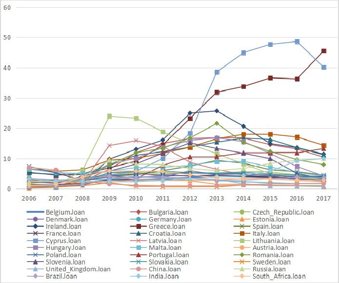
Sustainability 2020, 12, 747                                                                         2 of 20

limited. Meanwhile, there are many concurrent events that occur around sovereign defaults or crises.
Since the end of 2009, the increase of higher sovereign risk has pushed up the cost and affected the
financing structure of some euro area banks. The banks of Greece, Ireland, and Portugal find it difficult
to raise large-scale debt and deposits. It is very difficult to isolate the actual impact of sovereign debt
distress on bank loan distress from these concurrent events.
      In this study, we adopt three copula models to analyze the tail dependence between sovereign
debt distress and bank loan performance. Specifically, we use the ratio of government debt to Gross
Domestic Product (GDP) to measure sovereign debt exposure and the ratio of non-performing loans to
proxy for bank loan performance. The right tail of sovereign debt exposure and bank NPLs reflects the
likelihood of sovereign debt and bank loan distress, respectively. In contrast to the related studies [2–5]
that use actual sovereign debt defaults (or crises), our measures mitigate the impact of other concurrent
events around actual fiscal or financial crises and also significantly increase the sample size in term of
time span and countries. In particular, our study covers 25 countries during a period from 2006 to 2017.
      First, a Granger causality test was applied to examine the causality between sovereign debt and
bank NPLs. We find that most of the significant causality relationship occurs in the first-year lag
variables. For instance, the first-year lag of sovereign debt ratio significantly causes bank NPLs in
many countries, such as Cyprus, Portugal, Spain, Germany, Slovakia, Denmark, South Africa, etc.
Furthermore, we use Kendall’s tau as an alternative measure to exhibit the relationship between each
pair of countries in our sample. In particular, we divide our countries into two groups: European
countries and BRICS countries (Brazil, Russia, India, China and South Africa). We find that the mean
of Kendall’s tau among the European countries is about 0.4742, while the mean among the BRICS
countries is only 0.0141. This evidence suggests that geographical location is one of the factors affecting
the spillover effects of sovereign debt on bank NPLs.
      To analyze the asymmetry of the tail dependence structure between sovereign debt and bank
NPLs, we employ three of the most frequently used copula models in finance [7]: Student’s t-copula
(symmetric association of tail dependence), rotated Clayton copula (upper-tail dependence), and
Joe copula (upper-tail dependence). We employ these copulas because they are able to analyze the
upper tail dependence. Our empirical results suggest that the tail dependence between sovereign debt
and bank NPLs varies across countries. Most tail dependence results are consistent across the three
copula approaches with slight variation, especially in the t copula. All copula approaches point out
that the highest tail dependence between sovereign debt ratio and bank NPLs ratio occurs in Ireland
and Croatia. In addition, the tail dependence is high in Denmark, Belgium, Cyprus, Latvia, Austria,
and Portugal in contrast to other countries in our sample.
      Last, since the bank NPLs ratio is affected by many factors simultaneously, we use the Gaussian
copula regression method (GCRM) to isolate the important impact of sovereign debt on bank NPLs from
other known determinants. Particularly, we control GDP, inflation rate, government fiscal expenditure
and government fiscal revenue. We document significant and positive relation between sovereign
debt ratio and bank NPLs ratio in 15 out of 25 countries, which adds more credence to the upper tail
dependence between sovereign debt distress and bank non-performing loans in some countries, such
as Ireland and Croatia.
      This research contributes to the related literature from at least two aspects. First, we use a new
method to analyze the upper tail dependence between sovereign debt and bank NPLs. Most closely
related literature uses classical regression models to examine the relation between sovereign debt
defaults and financial crises [8–11]. In contrast to the classical regression models, copula models have
an advantage of analyzing the tail dependence between two distributions. For instance, Reboredo and
Ugolini use the CoVaR-copula approach and vine-copula conditional VaR approach to analysis the
impact of the European debt crisis on the banking risk in debt markets [12,13]. In this study, we use
three alternative copula approaches to explore the tail dependence between sovereign debt ratio and
bank NPLs ratio, which deepens the understanding of this relation.
Sustainability 2020, 12, 747 3 of 20
Second, our study enriches the literature on the determinants of bank NPLs by providing new
evidence from the aspect of macroeconomic factors. There is a long history and large amount
of literature to examine the determinants of bank NPLs. Most of the identified determinants are
microeconomic factors, mostly bank characteristics, such as cost efficiency [14]), bank’s risk management
function [15], government ownership [16], bank credit growth [17], etc. Recently, especially after the
sub-prime financial crises, a strand of literature has emerged to examine the impact of macroeconomic
and policy-related factors on bank non-performing loans, including monetary policy [18], inflation
rate [19,20], GDP [10,21,22], fiscal expenditure and revenue [23–26], unemployment rates and housing
price index [27], and policy rates [28,29]. Makri et al. reveal strong correlations between NPLs and
public debt of Eurozone’s banking systems for the period 2000–2008, and fiscal problems may raise
bad loans in this region [11]. Ghosh finds that liquidity risk, greater capitalization, greater cost
inefficiency, poor credit quality, and banking industry size significantly increase bank non-performing
loans. Similarly, inflation, state unemployment rates, and US public debt significantly increase bank
non-performing loans [27]. In contrast to previous studies, this paper identifies a new macroeconomic
factor, sovereign debt to GDP ratio, which affects bank NPLs ratios. Empirical evidence shows that the
impact of sovereign debt ratio on bank non-performing loans varies across countries. Liu et al. find
that the government debt and NPLs of EU and BRICS countries increased drastically after the crisis,
and crisis countries are contagious [30].
The organization of this paper is as follows: Section 2 describes the econometric methodology in
the analysis. Section 3 defines the variables and data descriptions. Section 4 discusses the empirical
results. Finally, Section 5 concludes.
2. Econometric Methodology
2.1. Granger Causality Tests
Granger causality shows that the lagged value of one variable is conducive to predicting another
variable [31]. To study the causality relationship between sovereign debt and bank NPLs, we follow
the Granger causality test to analyze the existence of a causality relationship. More precisely, we plan
to test whether the change of sovereign debt precedes NPLs or, on the contrary, whether NPLs precede
the sovereign debt (and even whether these relationships are bidirectional).
Consider two variables, Xt and Yt , Xt Granger-causes Yt suggested that lags of Xt provide useful
information to explain present values of Yt and vice versa. Under these conditions, the Granger
causality model is as follows:
k
X k
X
Xt = ϕ1 + a1i Xt−i + b1 j Yt− j + ε1t (1)
i=1 j=1
k
X k
X
Yt = ϕ2 + a2i Xt−i + b2 j Yt− j + ε2t (2)
i=1 j=1
where X and Y denote NPLs and sovereign debt, interchangeably; ϕ1 and ϕ2 are the intercepts of
the equation; and k is the lag length. a and b represent estimation coefficients, and ε denotes error
terms. This model is suitable for testing the causality relationships between NPLs and sovereign debt
during 2006–2017. For each sample country, alternative causal relationship can be found [32]. There
is a one-way Granger-causality from X to Y if not all b2 j are zero, but all a1i are zero. Similarly, there
is a one-way Granger-causality from Y to X if not all a2i are zero, but all b1 j are zero. Additionally,
there is a two-way Granger-causality between X and Y if all b2 j and a2i are not zero. There is no
Granger-causality between X and Y if b2 j and a2i are zero [33].Sustainability 2020, 12, 747 4 of 20
2.2. Kendall’s Tau Coefficient
In statistics, Kendall’s tau coefficient is a measure of nonlinear dependence between two random
variables X and Y, which was put forward by Maurice Kendall in 1938. Kendall’s tau shows that there
is a monotonic (but not necessarily linear) relationship between the two variables. A Kendall’s tau test
is a nonparametric hypothesis test based on the tau correlation coefficient [34].
According to Kendall, suppose a pair of points (Xi , Y j ) and (X j , Y j ) are considered to be concordant
if Xi < X j and Yi < Y j or if Xi > X j and Yi > Y j , meaning that the pairs are in the same order to each
variable. Namely, a higher value of X corresponds to a higher value of Y; on the contrary, a lower
value of X corresponds to a lower value of Y. The pairs are considered to be discordant if Xi < X j
and Yi > Y j or if Xi > X j and Yi < Y j , meaning that the values of variables are arranged in opposite
directions; in other words, a lower value of X corresponds to a higher value of Y, and a higher value of
X corresponds to a lower value of Y [35,36]. The pairs are tied if Xi = X j and/or Yi = Y j .
If two random variables X and Y obey joint distribution H (x, y) and two vectors of (Xi , Yi ) and
(X j , Y j ) are independent, then Kendall’s tau is defined by
τ = P[(Xi − X j )(Yi − Y j ) > 0] − P[(Xi − Y j )(Xi − X j ) < 0] (3)
Equation (3) will calculate a value in [−1,1], which is the same as Pearson’s correlation. The higher
the absolute value of τ, the stronger the correlation between the two variables. Specifically, a positive
value indicates that the higher value of one variable is associated with the higher value of another
variable, and a negative value is the opposite [37].
2.3. Copula Function and Tail Dependence
Copulas were first introduced in the Sklar theorem and further developed by Joe (1997). A copula
is a function that relates univariate distribution to one-dimensional marginal multivariate distribution
of related variables
H (x, y) = C(FX (x), FY ( y)) (4)
where H (.) is a bivariate function, and FX (.) and FY (.) are cumulative distribution functions of X and Y.
Sklar’s theorem says that univariate margins can be separated from the dependence structure, and the
dependency structure can be represented by a copula, which is C [38]. A bivariate copula is a function
C: [0,1]2 → [0,1], which has the following properties, that is, u = FX (x) and v = FY ( y):
(1) The domain of C(u, v) is [0,1] × [0,1]
(2) C(u, 1) = C(1, u) = u, C(v, 1) = C(1, v) = v, ∀u, v ∈ [0,1]
(3) C(u, v) has zero fundamentals and is incremented in two dimensions
As can be seen from the above definition, copulas are a useful way to model dependent
random variables. Copulas have some certain properties that are very useful in dependency studies.
Firstly, copulas are always constant for strictly increasing the transformation of random variables.
Secondly, consistency measurements between widely used random variables, such as Kendall’s tau
and Spearman’s rho, are attributes of copulas. Thirdly, tail dependence is also an attribute of copulas.
Nelsen defines the upper and lower tail dependence coefficients for τU ∈ [0, 1] and τL ∈ [0, 1] of
(X, Y) [39]
τU = lim P[U > ε|V > ε ] = lim P[V > ε|U > ε ]
ε→1 ε→1
(5)
τL = lim P[U ≤ ε|V ≤ ε ] = lim P[V ≤ ε|U ≤ ε ]
ε→0 ε→1
The upper (right) and lower (left) tail dependence of a normal copula are equal, which is
τL = τU = 0, and this means that variables are independent in the extreme of distribution. The most
common assumption is the normal copula in finance although it does not have tail dependence. There
are many types of copulas that have left or right tail dependence.Sustainability 2020, 12, 747 5 of 20
2.3.1. Student’s t Copula
Similar to the normal distribution, the t distribution is a symmetrical bell-shaped distribution,
but its tail is heavier, which means it is more likely to produce values far below its mean [40].
Tλ −1 (u) Z Tλ−1 (v)
− λ+2 2
s2 + r2 − 2ρrs
Z
1
Ct (u, v ρ, λ ) =
1 + dsdr (6)
λ(1 − ρ)2
p
2π 1 − ρ2
−∞ −∞
where λ denotes the degrees of freedom of the t copula, ρ is the coefficient of linear correlation,
and Tλ−1 is the inverse of the standard univariate t-distribution function with λ degrees of freedom.
2arcsinρ
The Kendall’s tau of the t copula is π , and
√ √ !
k +1 1−ρ
τL = 2 − 2tk+1 √
1+ρ
√ √ ! (7)
k +1 1−ρ
τU = 2 − 2tk+1 √
1+ρ
√ √ !
− k+1 1−ρ
where tk+1 √ represents the value of the standard t-distribution function with the degree of
1−ρ
√ √ !
− k+1 1−ρ
freedom k + 1 at √ .
1−ρ
2.3.2. Clayton Copula
Clayton proposed one of the first bivariate association models for survival analysis [41]. Especially,
the Clayton copula is a popular method for time dependent association data, and it has a lower tail
dependence between variables and can fit structural relationships with lower tail dependence well;
it is higher for negative events than joint positive events.
−1/θ
C(u, v|θ ) = (u−θ + v−θ − 1) (8)
α
where ∀θ ∈ (0, ∞), the Kendall’s tau of the Clayton copula is 2+α , and τL = 2−1/α .
2.3.3. Joe Copula
In order to estimate the copula from a bivariate observational data set, Joe proposed the tail
dependence concept with copulas [42]. It relates the amount of dependence of the upper-right quadrant
tail or the lower-left quadrant tail of a bivariate distribution. The upper tail dependence that can be
found by the Joe copula is defined by
i1/θ
C(u, v|θ ) = 1 − (1 − u)θ + (1 − v)θ − (1 − u)θ (1 − v)θ
h
(9)
where θ ∈ [1, ∞).
2.4. Gaussian Copula Regression Method
Linear regression has been extensively used by statisticians to find the relationship between
dependent variables [43]. However, the assumption of linear relationship is too unrealistic and
restrictive in real application. Copula regression is more suitable than a linear model when the
dependent variable does not follow a normal distribution. Gaussian copula regression has been
increasingly popular in longitudinal data analysis, time series, mixed data, and spatial statistics.
Copula regression uses various copula models to represent the joint distribution of a pair of continuous
and discrete random variables. The marginal can be defined by various parametric distributions. The
marginal distributions are fitted to the bivariate joint distribution by maximum likelihood [44,45].Sustainability 2020, 12, 747 6 of 20
To avoid the multicollinearity in regression analysis, we employ the Gaussian copula marginal
regression (GCMR) for each country to measure the macroeconomic variables to assess the impact
on NPLs.
Consider a vector of n dependent variables Y1 , . . . , Yn . Let F(·|xi ) be the marginal cumulative
distribution of Yi for covariates xi . The joint data cumulative distribution function in the Gaussian
copula regression is expressed as
Pr(Y1 ≤ y1 , . . . , Yn ≤ yn ) = Φ(τ1 , . . . , τn ; P) (10)
where τi = Φ−1 F( yi |xi ) . For the correlation matrix of P, Φ(·) represents the univariate standard normal
cumulative distribution function and Φ(·; P) denotes the multivariate standard normal cumulative
distribution function. More details of the Gaussian copula model are described in Song [46] and
Masarotto [47]. In particular, an equivalent formulation of the Gaussian copula is given by
Yi = h(xi , τi ) (11)
where τi represents a stochastic error. The Gaussian copula regression model assumes that
h(xi , τi ) = F−1 Φ(τi )|xi
(12)
and the vector of errors τ = (τ1 , . . . , τn )T follows multivariate normal distribution.
To avoid linearity, normal and independent assumptions, Gaussian marginal distributions for
individual predictor variables are used with Gaussian copula functions in this paper.
NPLs ratiot = β0 + β1 × government − to − GDP ratiot + β2 × Expendituret +
(13)
β3 × GDPt + β4 × Revenuet + µt
where µt is the error term, µt = ϕµt−1 + ωt , and ωt ∼ iidN (0, σ2ω ) for the GCMR.
3. Definition of Variables and Data Description
3.1. Variables and Data Description
In this paper, we investigate tail dependence between sovereign debt distress and bank NPLs.
The data are comprised of general government gross debt to GDP ratio, bank NPLs, GDP, government
fiscal expenditure, government fiscal revenue, and inflation rate which are retrieved from Eurostat
and the International Monetary Fund (IMF). Table 1 presents macroeconomic variables in this study
and their corresponding sources. We exclude these countries in the sample because data availability
problems in some countries, such as Luxembourg, the Netherlands, and Finland. The final sample
includes 30 countries, including 25 EU countries and 5 BRICs countries. This paper covers the period
of 11 years (2006–2017), which includes both the global financial crisis and European sovereign debt
crisis period.
As can be seen from Figures 1 and 2, there are similar fluctuations of two key variables between
most sample countries. Meanwhile, the rise of the bank non-performing loan ratio is often accompanied
by the expansion of general government gross debt. This feature provides evidence that a dependence
of two key variables may exist.Sustainability 2020, 12, 747 7 of 20
Table 1. Definition of variables used in this paper.
Variable Definition Source
Non-performing loans The ratio of non-performing loans to total Eurostat, International
(NPLs) loans. Monetary Fund (IMF)
The general government gross debt to GDP
Sovereign debt Eurostat, IMF
ratio.
GDP has a significant negative impact on
NPLs, because the growth of GDP creates
Gross domestic product more jobs, which increases income of
IMF
(GDP) borrowers and reduces NPLs. Therefore,
the level of NPLs will rise when the
economy slows down.
It is represented by a percentage change in
regional consumer price index (CPI) and
low liquidity level is conducive to economic
Inflation rate IMF
growth, while high liquidity rate weakens
borrowers’ solvency by reducing their real
income, thus increasing NPLs.
Government fiscal expenditure refers to the
funds expended by the government.
Economic growth through fiscal
expenditure and government investment, as
well as more central government deficits
Government fiscal
and money supply has been greatly limited IMF
expenditure
after the economic crisis. Meanwhile,
insufficient fiscal revenue will offset the
growth of tax revenue. When the
government faces a budget deficit, it will
generate public debt.
Government revenue is the income
available to fund the activities of a
government. High fiscal revenue usually
means the government controls a large
Government fiscal revenue IMF
share of financial resources has the ability to
repay bank loans, while fiscal distress
implies that fiscal revenue cannot satisfy
government’s expenditures.
From Figure 1, it is obvious that the NPLs ratio of the sample countries experienced a huge
fluctuation during 2007–2017. After the global financial crisis of 2008, the bank non-performing loan
ratio changed significantly for many EU countries such as Greece, Cyprus, Lithuania, Ireland, Latvia,
Italy, Croatia, Bulgaria, Hungary, Portugal, Malta, Romania, et al. Meanwhile, the scale of the NPLs
ratio expanded significantly when the European sovereign debt crisis emerged. After the debt crisis’
peak in 2013, the NPLs ratio started to decrease in most sample countries. One of the important events
of the Greek crisis occurred on 18 October 2009 when the Greek government announced that the
budget deficit had increased to at least 12% of the GDP, double the government’s estimate. The NPLs
ratio of Cyprus and other EU countries rose sharply when the Greek government bonds defaulted,
as those countries’ banks invested heavily in Greek sovereign debt. Therefore, the economic crisis did
spread to countries such as Portugal, Italy, Ireland, Spain, France, and other countries with strong
economic strength in the Eurozone. However, the NPLs ratio for the non-crisis countries (Estonia,
Sweden, Germany, China, Brazil, South Africa, et al.) remained relatively stable after the outbreak of
the crisis. It cannot be ignored that the non-performing loan ratio of the banks in two BRICS countries
(India and Russia) has been continuously increasing.Sustainability 2020, 12, 747 8 of 20
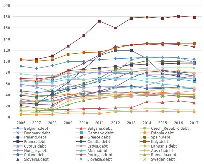
Figure 2 shows the government-to-GDP ratio for each of the sample countries in the sample. The
evolutions of these ratios are very similar; thus, we can distinguish some different periods marked by
the global financial risk of 2008 and the European sovereign debt crisis of 2009. It can be seen that
the government-to-GDP ratio of most sample countries is lower than the 90% debt cliff before 2007.
As the global financial crisis deepened, the government-to-GDP ratio began to largely increase in all of
the sample countries, especially in Greece, Italy, Portugal, Ireland, and Belgium. By the end of 2017,
the government-to-GDP ratio of Greece reached 180.8%, three times the Eurozone government-to-GDP
ratio limit set at 60%. Lately, Belgium, Spain, Cyprus, Slovenia, and the United Kingdom also show
large increases. Different from the bank non-performing loan ratio, the government-to-GDP ratio of
the BRICS countries such as China, Brazil, and South Africa has grown slowly since 2008. However,
the government-to-GDP ratio of Brazil and India has reached above 69%, higher than some EU countries
(Sweden, Slovakia, Lithuania, et al.). Large government debt in many sample countries (developed
economics and underdeveloped economics) has become a serious problem.
Sustainability 2020, 12, 747 8 of 9
Figure 1. Bank non‐performing
Figure 1. non-performing loans
loans (NPLs)
(NPLs) ratio
ratio of
of the
the sample
sample countries
countries since
since during
during 2007–2017.
2007–2017.
Source: Eurostat; International Monetary Fund.
From Figure 1, it is obvious that the NPLs ratio of the sample countries experienced a huge
fluctuation during 2007–2017. After the global financial crisis of 2008, the bank non‐performing loan
ratio changed significantly for many EU countries such as Greece, Cyprus, Lithuania, Ireland,
Latvia, Italy, Croatia, Bulgaria, Hungary, Portugal, Malta, Romania, et al. Meanwhile, the scale of
the NPLs ratio expanded significantly when the European sovereign debt crisis emerged. After the
debt crisis’ peak in 2013, the NPLs ratio started to decrease in most sample countries. One of the
important events of the Greek crisis occurred on 18 October 2009 when the Greek government
announced that the budget deficit had increased to at least 12% of the GDP, double the
government’s estimate. The NPLs ratio of Cyprus and other EU countries rose sharply when the
Greek government bonds defaulted, as those countries’ banks invested heavily in Greek sovereign
debt. Therefore, the economic crisis did spread to countries such as Portugal, Italy, Ireland, Spain,
France, and other countries with strong economic strength in the Eurozone. However, the NPLs
ratio for the non‐crisis countries (Estonia, Sweden, Germany, China, Brazil, South Africa, et al.)
remained relatively stable after the outbreak of the crisis. It cannot be ignored that the non‐
performing loan ratio of the banks in two BRICS countries (India and Russia) has been continuouslySustainability 2020, 12, 747 9 of 20
Sustainability 2020, 12, 747 9 of 10
Figure 2. Government‐to‐gross
Figure 2. Government-to-gross domestic
domestic product
product (GDP)
(GDP) ratio
ratio of
of the
the sample
sample countries
countries since
since during
during
2007–2017. Source: Eurostat; International Monetary Fund.
2007–2017. Source: Eurostat; International Monetary Fund.
3.2. Descriptive Statistics
Figure 2 shows the government‐to‐GDP ratio for each of the sample countries in the sample.
The evolutions
Basic summary of these ratios are
descriptive very of
statistics similar; thus, we
key variables canindistinguish
used this paper are some different
presented periods2
in Tables
marked by the global financial risk of 2008 and the European sovereign debt
and 3. The mean is significantly different from zero for the NPLs ratio and government-to-GDP crisis of 2009. It can be
ratio
seen
in thethat the countries.
sample government‐to‐GDP
As shown, ratio of most
the average ofsample countries
some sample is lower
countries than the
is higher than90%
other debt cliff
sample
before 2007. As the global financial crisis deepened, the government‐to‐GDP ratio
countries. The reason is simply that as the European sovereign debt crisis unfolded, some countries with began to largely
increase in all of the sample
weak competitiveness and loosecountries,
financialespecially in Greece, as
supervision—such Italy, Portugal,
Greece, Cyprus, Ireland, and
Ireland, Belgium. By
etc.—widened
the
the end
means of in
2017, the 2government‐to‐GDP
Tables and 3 more speedilyratio thanofdid
Greece
BRICSreached 180.8%,
countries. Boththree times the Eurozone
the minimum/maximum
government‐to‐GDP ratio limit set at 60%. Lately, Belgium, Spain, Cyprus,
and the standard deviations indicate that there is a notable time series variation in the Slovenia, andkeythe United
variables.
Kingdom also show large increases. Different from the bank non‐performing
For example, the bank non-performing loan ratio for Greece reached a maximum of 45.57 basis points loan ratio, the
government‐to‐GDP
(see Table 2), and the ratio of the BRICS countries
government-to-GDP ratio forsuch as China,
Portugal Brazil,
reached and South
a maximum of Africa has grown
130.6 basis points
slowly since
(see Table 3). 2008. However, the government‐to‐GDP ratio of Brazil and India has reached above
69%, In
higher thantime
the same someperiod,
EU countries
the NPLs (Sweden,
ratio forSlovakia,
Cyprus andLithuania, et al.). Large government
the government-to-GDP ratio for debt in
Greece
many sample countries (developed economics and underdeveloped economics)
reached maximum values of 48.68 basis points and 180.8 basis points, respectively. Meanwhile, has become a
serious problem.
the mean values of the key variables are typically very close to the average values. As shown in Table 2,
negative values for skewness are more pronounced for the Czech Republic than for the other sample
3.2. Descriptive Statistics
countries, which suggests a bigger probability of large decreases, suggesting that those distributions
haveBasic summary
long left descriptivethere
tails. Meanwhile, statistics of keyofvariables
is evidence positive used in this
skewness forpaper areChina,
Sweden, presented inLatvia,
India, Table
2and
andLithuania
Table 3. The
and mean is significantly
therefore distributions different fromright
with long zerotails.
for the NPLs ratiothat
Considering andthe
government‐to‐
kurtosis of a
GDP
normalratio in the sample
distribution countries.
is generally As shown,
3, Table 2 showsthethat
average
mostof some
the sample countries
distribution is of
of kurtosis higher than
the NPLs
other
ratio issample countries.
lower than The reason
3, suggesting that is simply
it does notthat asathe
have European distribution.
heavy-tailed sovereign debt crisis unfolded,
some countries with weak competitiveness and loose financial supervision—such as Greece,
Cyprus, Ireland, etc.—widened the means in Table 2 and Table 3 more speedily than did BRICS
countries. Both the minimum/maximum and the standard deviations indicate that there is a notable
time series variation in the key variables. For example, the bank non‐performing loan ratio for
Greece reached a maximum of 45.57 basis points (see Table 2), and the government‐to‐GDP ratio for
Portugal reached a maximum of 130.6 basis points (see Table 3).Sustainability 2020, 12, 747 10 of 20
Table 2. Descriptive statistics for the bank non-performing loan ratio.
Mean Median Minimum Maximum St.D Skewness Kurtosis
Belgium 2.9642 3.1900 1.1600 4.2400 1.0694 −0.6117 2.0734
Bulgaria 10.7067 12.545 2.1000 16.8800 5.9127 −0.4996 1.6586
Czech
4.4858 4.8950 2.3700 5.6100 1.1010 −0.7795 2.2255
Republic
Denmark 3.1392 3.4800 0.4000 5.9500 1.6898 −0.3115 2.2255
Germany 2.6633 2.7800 1.6900 3.4000 0.5744 −0.4537 1.9127
Estonia 2.1083 1.4300 0.2000 5.3800 1.8157 0.8590 2.2676
Ireland 12.7833 13.3300 0.5300 25.7100 8.6392 −0.0637 2.0023
Greece 21.0450 18.8500 4.5000 45.5700 15.1776 0.2151 1.4648
Spain 5.0642 5.1200 0.7000 9.3800 2.7234 −0.1510 2.1743
France 3.6867 3.8700 2.7000 4.5000 0.6312 −0.3824 1.6509
Croatia 11.0725 11.7350 4.7500 16.7100 4.4540 −0.3116 1.6736
Italy 12.3108 12.7450 5.7800 18.0600 4.6595 −0.1378 1.5490
Cyprus 21.9842 14.1800 0.6000 48.6800 20.1756 0.2544 1.2686
Latvia 6.6000 4.6200 0.5000 15.9300 5.4205 0.6585 1.9852
Lithuania 10.0508 7.1350 1.0000 23.9900 8.3663 0.5788 1.8944
Hungary 9.3150 9.1400 2.3000 16.8300 5.4712 0.0334 1.5220
Malta 6.5892 6.7450 4.1000 9.05000 1.5497 0.1544 2.0655
Austria 2.6900 2.7250 1.9000 3.4700 0.4563 0.1258 2.4942
Poland 4.7175 4.7400 2.8200 7.4000 1.0769 0.8988 4.8279
Portugal 7.3750 9.1250 1.3000 13.3000 4.8475 0.1852 1.2605
Romania 10.3367 10.7600 1.8000 21.6000 6.1126 0.1340 2.1850
Slovenia 7.7317 7.0000 1.8000 15.1800 4.5795 0.2129 1.6299
Slovakia 4.4883 4.9850 2.5000 5.8000 1.2140 −0.6285 1.9133
Sweden 0.9758 0.9000 0.6000 2.0000 0.3941 1.4469 4.7866
United
2.1617 1.6250 0.8100 3.9600 1.3342 0.3073 1.3017
Kingdom
China 2.3125 1.6350 0.9500 7.1000 2.0789 1.6631 4.0742
Russia 6.8017 7.3650 2.4000 10.0000 2.6596 −0.5731 2.0161
Brazil 3.3600 3.3800 2.8500 4.2100 0.4157 0.6093 2.5971
India 4.3675 3.3350 2.3000 9.9800 2.6547 1.2948 3.2111
South
3.6742 3.4350 1.1000 5.9000 1.5988 −0.0098 2.0376
Africa
Table 3 reports summary statistics for the general government gross debt of the sample countries.
Average means close to zero, which is like the bank non-performing loan ratio. Negative values for
skewness are more pronounced for Latvia, Hungary, and Belgium, suggesting that those distributions
have long left tails. Meanwhile, there is evidence of positive skewness for Sweden, Brazil, China,
and India and therefore of distributions with long right tails. EU countries (except Sweden) have
negative values for skewness, whereas the five BRICS countries have opposite results. The distribution
of the kurtosis of the government-to-GDP ratio does not comply with the normal distribution generated
from Table 3.Sustainability 2020, 12, 747 11 of 20
Table 3. Descriptive statistics for the government-to-GDP ratio.
Mean Median Minimum Maximum St.D Skewness Kurtosis
Belgium 100.3583 102.8500 87.0000 107.0000 6.6701 −0.8902 2.4051
Bulgaria 19.6333 16.8500 13.0000 29.0000 5.7362 0.4649 1.6080
Czech
36.4417 37.1000 27.5000 44.9000 6.2432 −0.2141 1.7903
Republic
Denmark 39.0333 40.0500 27.3000 46.1000 5.9322 −0.6277 2.2842
Germany 71.9000 71.8000 63.7000 80.9000 6.3577 0.0684 1.5050
Estonia 7.6083 8.0000 3.7000 10.7000 2.5300 −0.2885 1.5525
Ireland 75.7500 74.8500 23.6000 119.6000 34.0440 −0.2120 1.8718
Greece 151.1000 165.8500 103.1000 180.8000 31.9020 −0.5597 1.6123
Spain 72.8917 77.6000 35.6000 100.4000 26.4605 −0.2630 1.4036
France 85.1750 89.2000 64.5000 97.0000 12.4362 −0.7907 2.0593
Croatia 63.3833 66.6000 37.3000 84.0000 18.6716 −0.2974 1.4865
Italy 119.0583 119.9500 99.8000 132.0000 12.6018 −0.3452 1.5921
Cyprus 77.8750 72.7000 45.1000 107.5000 24.8807 0.0977 1.2836
Latvia 33.3000 39.5500 8.0000 46.8000 13.3813 −1.1015 2.5721
Lithuania 32.5500 38.0000 14.6000 42.6000 10.6798 −0.8592 1.9943
Hungary 74.8750 76.6500 64.5000 80.5000 5.2343 −1.0305 2.8415
Malta 63.3583 64.1500 50.8000 70.1000 5.7175 −0.9038 2.9411
Austria 78.3167 81.6000 65.0000 84.6000 7.0776 −1.0123 2.3322
Poland 50.8000 50.8500 44.2000 55.7000 3.5868 −0.4349 2.0792
Portugal 105.8917 118.5500 68.4000 130.6000 26.2724 −0.4422 1.4574
Romania 28.8333 34.5000 11.9000 39.1000 11.0311 −0.7188 1.7858
Slovenia 52.4583 50.2000 21.8000 82.6000 23.7567 −0.0003 1.3967
Slovakia 43.8500 47.3000 28.5000 54.7000 10.0848 −0.4233 1.5416
Sweden 40.8500 40.6500 37.8000 45.5000 2.6586 0.4120 1.8766
United
72.9333 82.9000 40.8000 88.2000 18.7544 −0.8410 2.0280
Kingdom
China 35.6000 34.3000 25.4000 47.6000 6.7618 0.1938 2.1800
Russia 11.5417 11.3500 7.4000 15.9000 2.6569 0.1562 2.2124
Brazil 58.4508 56.1300 51.2700 74.0400 7.4771 1.0211 2.7483
India 70.7583 69.5500 67.5000 77.1000 3.0125 0.9404 2.5640
South
39.9167 39.6000 27.8000 53.1000 9.0799 0.0783 1.5803
Africa
4. Empirical Results and Discussion
4.1. Granger Results
Table 4 reports the p-values for Granger causality between NPLs and sovereign debt at various
levels of lags in the 30 countries. We observe a bi-directional causality relationship in Cyprus,
Italy, Portugal, Romania, Spain, Denmark, Sweden, and South Africa. It cannot be ignored that the
bi-directional causal link is mainly found in northern and southern European countries. In those
countries, the evidence for bi-directional causality is consistent with the evolution of sovereign debt
and NPLs. A substantial increase in the size of sovereign debt occurred in the outbreak of the financial
crisis, suggesting a strong interaction between sovereign debt and NPLs.
It can also be observed that unidirectional causality occurs? between NPLs and sovereign debt
for Bulgaria, Greece, Malta, Slovenia, Ireland, United Kingdom, Austria, Czech Republic, Germany,
Lithuania, Brazil, and India. Our results show that there are several countries for which the null
hypothesis of causality between sovereign debt and NPLs cannot be rejected, including Greece, Malta,
Slovenia, Ireland, Austria, Czech Republic, Germany, Lithuania, Brazil, and India. The debt ratio rises
significantly in the European countries after the recent European debt crisis. Considering the obviously
low return on debt accumulation, it seems to have exacerbated the scale of NPLs. Note that Brazil and
India are emerging countries with a strong willingness to lend. Nevertheless, we find that bank NPLsSustainability 2020, 12, 747 12 of 20
cannot significantly cause the change of sovereign debt in Bulgaria and the United Kingdom at the
conventional level.
A causal relationship exists between sovereign debt and NPLs since the non-causality null
hypothesis is rejected in Croatia, Belgium, France, Hungary, Poland, Estonia, Latvia, China, and Russia.
Statistical evidence exists against the null hypothesis of an absence of causal relationship between
sovereign debts and debt in sample countries, especially in Western Europe, central Europe, and Eastern
European countries. It is important to recall that their economic problems have been merged after the
economic crisis and sovereign debt crisis.
Table 4. Granger causality test for the lag ki (i = 1,2,3).
Debt → NPLs NPLs → Debt
Country
k=1 k=2 k=3 k =1 k=2 k=3
Belgium 0.0690 0.0928 0.1287 0.0621 0.06772 0.2773
Bulgaria 0.1033 0.4841 0.9006 0.0085 ** 0.0767 0.3815
Czech
0.0398 * 0.0362 * 0.1691 0.1746 0.2878 0.2525
Republic
Denmark 0.0056 ** 0.598 0.9068 0.0001 *** 0.0133 * 0.0907
Germany 0.0011 ** 0.1085 0.0445 * 0.0928 0.0587 0.2920
Estonia 0.4735 0.2668 0.1499 0.1239 0.3308 0.1546
Ireland 0.7105 0.0138 * 0.2595 0.2626 0.6566 0.7956
Greece 0.0102 * 0.0347 * 0.1988 0.9357 0.5671 0.2092
Spain 0.0028 ** 0.5248 0.1932 0.0024 ** 0.0358 * 0.1492
France 0.4955 0.8559 0.6277 0.1203 0.2864 0.7300
Croatia 0.1952 0.1818 0.1523 0.9109 0.8177 0.7420
Italy 0.3479 0.0128 * 0.1527 0.1608 0.0003 *** 0.2963 *
Cyprus 0.0003 *** 0.5192 0.6840 0.0042 ** 0.0109 * 0.8223
Latvia 0.9098 0.3147 - 0.8794 0.3847 0.0400 *
Lithuania 0.0089 ** 0.0042 ** 0.0638 0.1923 0.3646 0.6983
Hungary 0.6667 0.9697 0.6400 0.4286 0.2949 0.3772
Malta 0.0177 * 0.0599 0.3195 0.02565 0.6050 0.2901
Austria 0.01399 * 0.0352 * 0.031 * 0.1153 0.3596 0.8432
Poland 0.4803 0.6403 0.6308 0.6490 0.2583 0.4747
Portugal 0.0014 ** 0.2132 0.4841 0.0279 * 0.4442 0.8346
Romania 0.0245 * 0.1286 0.5888 0.036 * 0.0515 0.3409
Slovenia 0.4660 0.2373 0.0443 * 0.8733 0.8929 0.8374
Slovakia 0.0089 ** 0.0171 * 0.1097 0.2338 0.7354 0.7900
Sweden 0.0044 ** 0.3647 0.8736 0.0052 ** 0.1596 0.0232 *
United
0.4964 0.6775 0.8912 0.0009 *** 0.0268 * 0.4423
Kingdom
China 0.0948 0.0870 0.4707 0.7309 0.7335 0.0995
Russia 0.6297 0.5957 0.0577 0.8246 0.6897 0.2555
Brazil 0.2648 0.0435 * 0.3470 0.1724 0.1267 0.3427
India 0.0074 ** 0.2449 0.3934 0.8505 0.5818 0.2473
South Africa 0.0047 ** 0.0022 ** 0.1917 0.0094 ** 0.0615 0.9620
Note: For Debt → Loan, H0: Debt does not cause Loan. ***, **, and * denote rejection of the null hypothesis at the 1,
5, and 10% significance level, respectively.
Although it is difficult to find commonality of the impact of sovereign debt on bank NPLs across
countries, we note that countries with high sovereign debt ratio are usually associated with higher
NPLs. An increase in NPLs reflects the deterioration of banks’ balance sheets and asset quality, which in
turn may reduce banks’ leverage or profits. Losses on government bonds weaken banks’ balance sheets
and increase financing costs. Meanwhile, countries with larger amounts of sovereign debt exhibit a
one-way causal relationship between bank NPLs and sovereign debt or bi-directional causality. It is
noteworthy that the different characteristics across countries and the heterogeneity in the results point
towards caution when making inferences about the relationship between sovereign debt and NPLs.Sustainability 2020, 12, 747 13 of 20
4.2. Kendall’s Tau Results
Kendall’s tau shows the correlation between each pair of sample countries. We categorize all
pairs of countries into two groups according to the geographical location: European countries and
other (BRICS) countries. Table 5 reports the means of Kendall’s tau between the government-to-GDP
ratio and the bank NPLs for the sample countries. First, within the European group, we calculate the
means of Kendall’s tau between each country and the other countries and report the results in Panel A.
Since sovereign debt crisis occurs in European countries, to easily understand the spillover effect of
sovereign debt crisis on the emerging countries, we calculate the means of Kendall’s tau between each
BRICS country and all European countries and report the results in Panel B. We find that the means of
tau within European countries are much higher than the means within BRICS countries.
Table 5. Mean of Kendall’s tau for the NPLs ratio and the government-to-GDP ratio.
Mean of NPLs Mean of Debt
Panel A: Kendall’s Tau within European Countries
25 EU countries 0.4742 0.5815
Belgium-24 EU countries 0.4390 0.6167
Bulgaria-24 EU countries 0.4695 0.3874
Czech Republic-24 EU countries 0.4292 0.4951
Denmark-24 EU countries 0.4475 0.3667
Germany-24 EU countries −0.0679 0.2402
Estonia-24 EU countries 0.2619 0.5377
Ireland-24 EU countries 0.4351 0.4182
Greece-24 EU countries 0.2847 0.5571
Spain-24 EU countries 0.4592 0.6435
France-24 EU countries 0.4425 0.5350
Croatia-24 EU countries 0.4328 0.6147
Italy-24 EU countries 0.3719 0.5701
Cyprus-24 EU countries 0.3231 0.5619
Latvia-24 EU countries 0.3388 0.3293
Lithuania-24 EU countries 0.2956 0.5814
Hungary-24 EU countries 0.4758 0.2210
Malta-24 EU countries 0.3593 0.0442
Austria-24 EU countries 0.3469 0.4761
Poland-24 EU countries 0.0438 0.4184
Portugal-24 EU countries 0.2968 0.6035
Romania-24 EU countries 0.4594 0.6086
Slovenia-24 EU countries 0.4517 0.5915
Slovakia-24 EU countries 0.3841 0.5610
Sweden-24 EU countries 0.1051 0.2437
United Kingdom-24 EU countries 0.2969 0.5610
Panel B: Kendall’s Tau between BRICS and European Countries
5 BRICS countries 0.0141 0.2582
China-25 EU countries −0.3992 0.4438
Russia-25 EU countries 0.1456 0.5874
Brazil-25 EU countries −0.0064 0.0387
India-25 EU countries 0.0700 −0.3436
South Africa-25 EU countries 0.2498 0.5006
This result is not surprising because there are strong commonalities among European countries,
such as currency, geographical location, culture, etc. In particular, the highest means of tau occur in
Hungary and Bulgaria, in contrast to other European countries. While in BRICS countries, although
the economy grows relatively fast in these countries, the business models and the engines of economy
are very different, which leads to a low mean of correlations among these countries. Moreover, we note
that the means of tau between each BRICS country and the European countries varies significantly.Sustainability 2020, 12, 747 14 of 20
For example, the mean of correlation between South Africa and the European countries is positive but
the mean between Brazil and the European countries is negative. The heterogeneity of correlations
across countries might be due to the variation of country characteristics, which is out of the scope
of this paper. Sovereign risk has a negative spillover effect on bank risk, and failure to fully protect
the banking system from the impact of serious domestic sovereignty is a reason to maintain good
public finances.
4.3. Copula Results
We consider three copula models to analyze the tail dependence between the government-to-GDP
ratio and the bank non-performing loan ratio: Student’s t copula (symmetric association of tail
dependence), rotated Clayton copula (upper-tail dependence), and Joe copula (upper-tail dependence).
In terms of tail dependence, these series copula models cover the major combinations of features
necessary to capture possible associations between the variables studied, and they are the most
commonly used copulas in finance [7].
The estimation results of the three copula models above are shown in Table 6. The t-copula
detects both upper and lower tail dependence at each sample country. Because of the symmetry of the
Student’s t distribution, the upper tail coefficient is generally equal to the lower tail coefficient. We find
that the highest dependence of upper tails occurs in Ireland, about 0.8778. The large and positive tail
dependence suggests a strong correlation between the extreme expansion of sovereign debt and the
sharp increase of bank NPLs. In addition, there are five countries in which the upper tail dependence
is greater than 0.5, including Denmark, Ireland, Croatia, Latvia, and Portugal.
Table 6. Tail dependence for different copulas with the NPLs ratio and the government-to-GDP ratio.
t Copula Rotated Clayton Copula Joe Copula
Country
Lower Upper Lower Upper Lower Upper
Belgium 0.4045 0.4045 0 0.8047 0 0.8115
Bulgaria 0.0015 0.0015 0 0.3241 0 0.3892
Czech
0.0917 0.0917 0 0.5971 0 0.6215
Republic
Denmark 0.7460 0.7460 0 0.7905 0 0.8002
Germany 0.0011 0.0011 0 0.2882 0 0.3599
Estonia 0.0001 0.0001 0 0.0000 0 0.0001
Ireland 0.8778 0.8778 0 0.9231 0 0.9237
Greece 0.2977 0.2977 0 0.7800 0 0.7887
Spain 0.1112 0.1112 0 0.6620 0 0.6751
France 0.1909 0.1909 0 0.1300 0 0.1185
Croatia 0.8252 0.8252 0 0.9011 0 0.9020
Italy 0.2979 0.2979 0 0.7379 0 0.7514
Cyprus 0.2074 0.2074 0 0.8356 0 0.8412
Latvia 0.6543 0.6543 0 0.7781 0 0.7830
Hungary 0.0620 0.0620 0 0.5273 0 0.5548
Malta 0.4359 0.4359 0 0.5465 0 0.5850
Austria 0.0817 0.0817 0 0.7646 0 0.7698
Poland 0.1781 0.1781 0 0.0000 0 0.0001
Portugal 0.7246 0.7246 0 0.7089 0 0.7266
Romania 0.1218 0.1218 0 0.6658 0 0.6762
Slovenia 0.0083 0.0083 0 0.3696 0 0.4003
Slovakia 0.0057 0.0057 0 0.2229 0 0.2468
Sweden 0.0096 0.0096 0 0.5883 0 0.6172
Russia 0.0048 0.0048 0 0.2807 0 0.3127
Brazil 0.0043 0.0043 0 0.5227 0 0.5571
Then, we use the rotated Clayton and Joe copulas as alternative methods to examine the upper
tail dependence between sovereign debt ratio and bank NPLs ratio. In contrast to the Student’s tSustainability 2020, 12, 747 15 of 20
distribution, the underlying distributions in the rotated Clayton copula and Joe copula focus on the
upper tail dependence. According to Table 6, we note that the tail dependence levels in all countries
are consistent in the rotated Clayton and Joe copulas but very different from the dependence in the t
copula. The highest upper tail dependence occurs in Ireland as well under both the rotated Clayton
and Joe copulas. We document 17 out of 25 countries whose value of upper tail dependence is greater
than 0.5 using either the rotated Clayton copula or Joe copula which are symmetric copula functions so
that those Archimedean copula functions cannot fit asymmetric distributed data well.
4.4. Gaussian Copula Regression Method Results
In previous sections, we focused on examining the causality using statistical methods without
controlling for the other determinants of bank NPLs. Related literature identifies many factors that
drive bank NPLs ratios, at both macro- and micro-levels [14–17,48]. To isolate the impact of other
known determinants, we employ the Gaussian copula regression method (GCRM) in this section. Since
we use the aggregated level of bank NPLs over total loans, we focus on the macroeconomic variables.
Specifically, we control for GDP, inflation rate, government fiscal expenditure, and government fiscal
revenue in Gaussian copula regressions.
Because of heterogeneity across countries, as shown in the previous analysis, we perform the
Gaussian copula regressions country by country and report regression results in Table 7. We find
positive and significant coefficients for sovereign debt ratio in 17 out of 25 countries, including Cyprus,
Greece, Croatia, Malta, Italy, Romania, Portugal, Slovenia, Spain, Ireland, Belgium, Germany, Hungary,
Czech Republic, Sweden, Slovakia, and Brazil. These positive and significant coefficients in a majority
of the countries provide further support for the positive impact of sovereign debt ratio on bank NPLs
ratios. This positive relationship highlights that fiscal stress could be a potential factor that deteriorates
bank loan performance. In addition, we also document negative and significant coefficients in several
countries including France, the United Kingdom, and South Africa.
Regarding the control variables, their coefficients vary across countries. First, the impact of the
GDP growth rate on bank NPLs ratios is mixed. On one hand, positive economic growth for each
economy indicates an increase in the wealth of private sector individuals, enterprises, and other
institutions, which results in a strong capability of repaying their respective debts and a decrease of
bank NPLs ratios. On the other hand, the expansion of the economy is usually associated with credit
booming. For instance, the credit bubble before the sub-prime financial crisis. The cheap credit during
the expansion of the economy sows the seeds for non-performing loans, which suggests a positive
relation between GDP growth and bank NPLs ratio. According to the results in Table 7, we find
positive and negative coefficients for GDP growth rate in 7 and 4 countries, respectively, while the
coefficients of GDP growth rate are insignificant in other countries.
Second, a high inflation rate is usually accompanied by an expansionary monetary policy. The
enlarged monetary base under an expansionary monetary policy increases the supply of loans. Under
such circumstance, banks are more likely to adopt an aggressive strategy for lending, which possibly
results in a higher level of non-performing loans. Thus, we expect a positive relationship between
inflation rate and bank NPL ratio. However, we only document significant and positive coefficients
for inflation rate in five countries. On the contrary, we find significantly negative coefficients for
inflation in eight countries. One of the possible explanations is that an increase in economic activity
leads to enhanced demand for loans, which in turn can cause higher lending rates. In addition,
increased economic activity can reduce defaults and increase deposits because it can make business
more profitable. However, tightening monetary policy can increase interest rates and make banks
be more inclined to attract customers with higher risks and compensate them for the high risk by
raising loan interest rates. These results are consistent with the studies by Were and Wambua [49] and
Ghosh [27].Sustainability 2020, 12, 747 16 of 20
Table 7. GCMR estimation results of the NPLs ratio to the government-to-GDP ratio.
Country Intercept Debt Expenditure GDP Revenue Inflation
44.8120 * −0.2404 0.4717 0.5576 −1.2776 * −1.2742 *
Bulgaria
(18.9509) (0.3626) (0.5271) (0.4915) (0.6131) (0.6076)
1.7552 *** 0.7646 *** −0.7424 0.1576 −0.2369 −0.5485
Cyprus
(0.0024) (0.0715) (0.5010) (0.5022) (0.5877) (0.8323)
53.0771 *** 0.2805 *** 0.3155 *** 0.0338 −1.0389 *** −0.2666 ***
Croatia
(0.0004) (0.0093) (0.0562) (0.0412) (0.062) (0.07863)
−118.6 *** 0.2387 ** 0.5013 1.2320 ** 1.8230 *** −0.3670
Greece
(0.0065) (0.0903) (0.2686) (0.3769) (0.5232) (0.6392)
−76.6442 *** 0.22266 *** 0.2701 0.2415 * 1.0594 *** −0.3310
Italy
(0.0014) (0.02853) (0.2545) (0.1127) (0.2863) (0.2282)
28.7748 * 0.3301 *** −0.0692 0.3674 *** 0.4126 −0.1790
Malta
(11.5029) (0.0796) (0.2348) (0.0684) (0.3108) (0.2387)
−4.1232 0.1813 *** 0.3222 * 0.0537 0.1857 −0.0917
Portugal
(12.4124) (0.0146) (0.1385) (0.1089) (0.2245) (0.1744)
−12.5478 0.6090 *** −1.1359 −0.3779 1.3277 * 1.1883 **
Romania
(20.7407) (0.0893) (0.8139) (0.2783) (0.5304) (0.4413)
−27.9760 ** 0.0699 *** 0.3601 −0.2669 0.3274 * 0.0860
Spain
(10.5332) (0.0135) (0.1946) (0.1958) (0.1546) (0.1712)
−131.3625 *** 0.1401 *** 0.1843 −0.4206 ** 3.0411 *** 0.8356
Slovenia
(21.3408) (0.033) (0.1469) (0.1370) (0.5862) (0.4637)
−19.6475 *** 0.04560 *** 0.2127 *** 0.0205 0.1381 ** −0.1122 ***
Belgium
(0.9114) (0.0096) (0.0235) (0.0221) (0.0279) (0.0212)
−42.1100 *** −0.0807 *** 0.7195 *** 0.0410 0.2384 *** 0.0857
France
(0.0005) (0.0096) (0.0678) (0.0713) (0.0697) (0.0971)
−9.76100 0.2519 *** −0.2364 *** 0.0107 0.4172 * −1.0583 *
Ireland
(5.3245) (0.0139) (0.0689) (0.0699) (0.2016) (0.4138)
United −35.2600 *** −0.0104 * 0.6023 *** 0.0595 0.3763 *** 0.00591
Kingdom (0.0009) (0.0051) (0.0418) (0.0528) (0.0433) (0.0802)
−38.1600 *** 0.0000 0.2473 *** 0.2690 *** 0.5744 *** −0.0910 ***
Austria
(0.0003) (0.9981) (0.0000) (0.0275) (0.0412) (0.0469)
Czech 23.0463 *** 0.2120 *** 0.0625 0.0931 *** −0.7161 *** −0.2335 ***
Republic (0.0009) (0.0147) (0.0389) (0.0281) (0.0456) (0.0445)
18.3133 *** 0.0187 * 0.1316 *** −0.0854 *** −0.5232 *** 0.2074 **
Germany
(0.0004) (0.0090) (0.0363) (0.0225 (0.0312) (0.0780)
−155.4512 *** 0.8237 *** 1.1118 * 0.5173 1.0447 0.1635
Hungary
(40.5536) (0.2018) (0.5583) (0.3618) (0.6036) (0.4481)
−49.4549 * 0.1730 0.5021* 0.0908 0.6117 −3.7770 *
Poland
(19.4889) (0.1054) (0.1993) (0.2431) (0.3446) (0.1628)
−4.06700 0.0981 *** 0.4829 *** 0.0273 −0.4233 *** 0.1052
Slovakia
(3.3320) (0.0171) (0.0775) (0.0385) (0.0788) (0.0874)
−21.8500 * 0.0696 0.4173 * 0.0754 −0.0008 −0.1979
Denmark
(1094) (0.0787) (0.1649) (0.0830) (0.1549) (0.1464)
−0.0660 0.1284 *** 0.0373 −0.0792 *** −0.1271 * 0.3247 ***
Sweden
(3.0839) (0.0226) (0.0594) (0.0212) (0.0508) (0.0950)
−48.8265 ** 0.0166 −0.4439 −0.0130 1.6916 0.5242
Estonia
(18.7886) (0.3587) (0.7987) (0.1615) (1.0694) (0.3737)
−212.5658 *** −0.1794 3.2445 *** 0.6411 *** 2.7942 ** 0.6060 ***
Latvia
(39.9114) (0.0922) (0.3430) (0.1166) (0.9595) (0.1792)
12.7869 0.1462 2.0778 *** −0.1690 −2.4429 * −0.3245
Lithuania
(35.3126) (0.1060) (0.3039) (0.1391) (0.9685) (0.3397)
14.7477 0.1116 0.1928 −0.0441 −0.8561 * 0.08932
China
(8.7543) (0.1435) (0.5110) (0.4064) (0.3772) (0.1556)
43.9618 −0.1486 0.0552 −0.1515 −1.0344 ** −0.1898
Russia
(25.632) (0.1724) (0.3749) (0.1686) (0.3970) (0.1067)
−7.6525 0.0515 * 0.0048 −0.1513 ** 0.2473 ** −0.0237
Brazil
(4.7255) (0.0227) (0.1067) (0.0466) (0.0774) (0.0685)
1.2336 −0.2745 1.1337 −0.0997 −0.0520 −0.8655 ***
India
(20.9252) (0.1432) (0.61111) (0.2197) (−0.5827) (0.1773)
4.9088 *** −0.133 *** 1.0070 *** 0.2845 ** −1.0491 *** 0.2123 *
South Africa
(0.0009) (0.0188) (0.0887) (0.1061) (0.1153) (0.0845)
Note: * Significance at 10% level. ** Significance at 5% level. *** Significance at 1% level. Standard errors are
in parentheses.You can also read