Aerosol particle depolarization ratio at 1565 nm measured with a Halo Doppler lidar
←
→
Page content transcription
If your browser does not render page correctly, please read the page content below
Atmos. Chem. Phys., 21, 5807–5820, 2021
https://doi.org/10.5194/acp-21-5807-2021
© Author(s) 2021. This work is distributed under
the Creative Commons Attribution 4.0 License.

Aerosol particle depolarization ratio at 1565 nm measured
with a Halo Doppler lidar
Ville Vakkari1,2 , Holger Baars3 , Stephanie Bohlmann4,5 , Johannes Bühl3 , Mika Komppula4 ,
Rodanthi-Elisavet Mamouri6,7 , and Ewan James O’Connor1,8
1 Finnish Meteorological Institute, Helsinki, 00101, Finland
2 Atmospheric   Chemistry Research Group, Chemical Resource Beneficiation,
North-West University, Potchefstroom, South Africa
3 Leibniz Institute for Tropospheric Research, Leipzig, Germany
4 Finnish Meteorological Institute, Kuopio, 70211, Finland
5 Department of Applied Physics, University of Eastern Finland, Kuopio, Finland
6 Department of Civil Engineering and Geomatics, Cyprus University of Technology, Limassol, Cyprus
7 ERATOSTHENES Centre of Excellence, Limassol, Cyprus
8 Department of Meteorology, University of Reading, Reading, UK

Correspondence: Ville Vakkari (ville.vakkari@fmi.fi)

Received: 28 August 2020 – Discussion started: 23 October 2020
Revised: 26 February 2021 – Accepted: 4 March 2021 – Published: 19 April 2021

Abstract. The depolarization ratio is a valuable parameter        1   Introduction
for lidar-based aerosol categorization. Usually, the aerosol
particle depolarization ratio is determined at relatively short
wavelengths of 355 nm and/or 532 nm, but some multi-              Aerosols and their interactions with clouds remain the largest
wavelength studies including longer wavelengths indicate          source of uncertainty in the Earth’s radiative budget (IPCC,
strong spectral dependency. Here, we investigate the capabil-     2013). Remote sensing measurements with lidars enable con-
ities of Halo Photonics StreamLine Doppler lidars to retrieve     tinuous long-term observations of the vertical distribution
the particle linear depolarization ratio at the 1565 nm wave-     of aerosol particles and clouds in the atmosphere, providing
length. We utilize collocated measurements with another li-       valuable information for improving our understanding of the
dar system, PollyXT at Limassol, Cyprus, and at Kuopio,           global climate system (e.g. Illingworth et al., 2015). Infor-
Finland, to compare the depolarization ratio observed by the      mation on the vertical distribution of aerosols is highly im-
two systems. For mineral-dust-dominated cases we find typ-        portant also for the aviation industry in case of hazardous
ically a slightly lower depolarization ratio at 1565 nm than at   aerosol emissions from for example volcanic eruptions (Hirtl
355 and 532 nm. However, for dust mixed with other aerosol        et al., 2020).
we find a higher depolarization ratio at 1565 nm. For pol-           Lidar measurements of aerosol optical properties at mul-
luted marine aerosol we find a marginally lower depolariza-       tiple wavelengths can be used to categorize elevated aerosol
tion ratio at 1565 nm compared to 355 and 532 nm. For mixed       layers into different types such as mineral dust, smoke, ma-
spruce and birch pollen we find a slightly higher depolariza-     rine aerosol or volcanic ash (e.g. Baars et al., 2017; Papa-
tion ratio at 1565 nm compared to 532 nm. Overall, we con-        giannopoulos et al., 2018). One of the most important param-
clude that Halo Doppler lidars can provide a particle linear      eters for such aerosol typing is the depolarization ratio, which
depolarization ratio at the 1565 nm wavelength at least in the    enables distinguishing spherical and non-spherical particles
lowest 2–3 km above ground.                                       from each other (e.g. Burton et al., 2012; Baars et al., 2017).
                                                                  Furthermore, the depolarization ratio can be used to quantify
                                                                  the contributions of different aerosol types to elevated layers
                                                                  (Mamouri and Ansmann, 2017). It is essential also for esti-

Published by Copernicus Publications on behalf of the European Geosciences Union.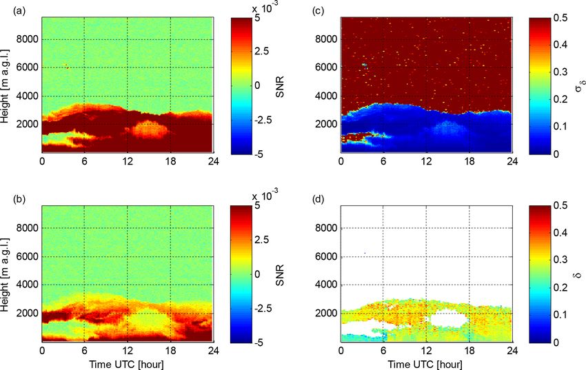
5808                                                                   V. Vakkari et al.: Aerosol particle depolarization ratio

mating vertical profiles of cloud condensation nuclei (CCN)
and ice-nucleating particle (INP) concentrations from remote
sensing observations (Mamouri and Ansmann, 2016).
   Currently, the particle linear depolarization ratio is most
commonly measured at relatively short wavelengths of 355
and/or 532 nm (e.g. Illingworth et al., 2015; Baars et al.,
2016), though some lidar systems are capable of depolar-
ization ratio measurement at longer wavelengths of 710 and
1064 nm (e.g. Freudenthaler et al., 2009; Burton et al., 2012).
For instance, Burton et al. (2012) used the ratio of depolar-
ization ratios at 1064 and 532 nm as part of their aerosol typ-
ing procedure. However, to our knowledge, the aerosol parti-
cle depolarization ratio has not been reported at wavelengths
longer than 1064 nm.
   Previous studies on the spectral dependency of the depo-
larization ratio between 355 and 1064 nm have shown a steep
decrease in the depolarization ratio from 532 to 1064 nm for       Figure 1. Locations of Vehmasmäki and Limassol measurement
elevated biomass burning aerosols (Burton et al., 2012, 2015;      sites.
Haarig et al., 2018; Hu et al., 2019). On the contrary, mineral
dust layers present an increasing depolarization ratio with in-
creasing wavelength (Groß et al., 2011; Burton et al., 2015)       al., 2015; Vakkari et al., 2015; Tuononen et al., 2017; Man-
or a relatively weak maximum at 532 nm (Freudenthaler et           ninen et al., 2018). Additionally, depolarization ratio mea-
al., 2009; Burton et al., 2015; Haarig et al., 2017). For some     surements by Halo lidars have been used to study cloud and
aerosol types, such as marine aerosol (Groß et al., 2011) and      precipitation phase (e.g. Achtert et al., 2015).
volcanic ash (Groß et al., 2012), no spectral dependency was          Now, recently developed post-processing (Vakkari et al.,
observed. However, volcanic ash mixed with boundary layer          2019) allows the utilization of significantly weaker signals
aerosol was observed with a clearly lower depolarization ra-       from Halo Doppler lidars than previously. Therefore, the
tio at 355 nm than at 532 nm (Groß et al., 2012).                  main aim of this paper is to assess the capabilities of Halo
   The spectral dependency of the depolarization ratio has         Doppler lidars in providing particle linear depolarization ra-
been attributed largely to the shape of the size distribution      tio measurements at the 1565 nm wavelength. To do so, we
of polarizing aerosol particles. In smoke layers, the depolar-     utilize collocated Halo Doppler lidar and multiwavelength
ization signal is probably due to non-spherical soot aggre-        Raman lidar PollyXT observations during two measurement
gates, which are in the size range of 100 nm to hundreds of        campaigns, where different polarizing aerosols were ob-
nanometres and thus do not produce a large depolarization          served. Overall, the comparison indicates that Halo Doppler
ratio at 1064 nm (Burton et al., 2015; Haarig et al., 2018;        lidars can add another wavelength at 1565 nm to studies on
Hu et al., 2019). Recently, Gialitaki et al. (2020) modelled       the spectral dependency of the particle linear depolarization
smoke as near-spherical submicron particles and found good         ratio, at least in the lowest 2–3 km above ground.
agreement with the observed spectral dependency of the de-
polarization ratio. On the other hand, mineral dust contains
significant amounts of coarse-mode particles (>1 µm in di-         2   Materials and methods
ameter), which can explain the large depolarization ratio also
observed at the 1064 nm wavelength (Freudenthaler et al.,          Here we use data from two measurement campaigns where
2009; Groß et al., 2011; Burton et al., 2015; Haarig et al.,       a Halo Photonics Doppler lidar and a PollyXT Raman lidar
2017). In aged dust layers, the faster removal of supermicron      were collocated: at Kuopio, Finland, from 9 to 16 May 2016
particles is thought to result in the depolarization ratio peak-   and at Limassol, Cyprus, from 21 April to 22 May 2017. The
ing at 532 nm (Freudenthaler et al., 2009; Groß et al., 2011;      campaigns represent quite different environments (Fig. 1)
Burton et al., 2015; Haarig et al., 2017). In other words, spec-   and enable the comparison of the depolarization ratio at
tral analysis of the depolarization ratio could permit more in-    1565 nm by the Halo instrument to the depolarization ratio at
depth diagnosis of coarse-mode polarizing aerosol.                 355 and 532 nm from PollyXT for a range of aerosol types.
   Halo StreamLine Doppler lidars are commercially avail-          Furthermore, the campaigns were equipped with different de-
able fibre-optic systems that operate at a wavelength of           vices of the Halo and PollyXT designs, and thus potential dif-
1565 nm and can be equipped with a cross-polar receiver            ferences between instrument individuals can be investigated.
channel for measuring the depolarization ratio (Pearson et            The Vehmasmäki site (62.738◦ N, 27.543◦ E; 190 m a.s.l.)
al., 2009). Over the last few years these lidars have become       in Kuopio is a rural location surrounded by boreal for-
widely used in wind and turbulence studies (e.g. Päschke et        est (Bohlmann et al., 2019). The focus of the campaign in

Atmos. Chem. Phys., 21, 5807–5820, 2021                                             https://doi.org/10.5194/acp-21-5807-2021
V. Vakkari et al.: Aerosol particle depolarization ratio                                                                            5809

May 2016 was to investigate the capability to characterize          Table 1. Specifications of Halo Doppler lidars used in this study.
the optical properties of airborne pollen with the multiwave-
length Raman lidar PollyXT (Bohlmann et al., 2019). Here,                 Wavelength               1565 nm
we utilize 1 week of collocated measurements to compare                   Pulse repetition rate    15 kHz
Halo depolarization at 1565 nm to PollyXT during a spruce                 Pulse energy             20 µJ
and birch pollination episode.                                            Pulse duration           0.2 µs
   Limassol (34.675◦ N, 33.043◦ E; 22 m a.s.l.) is located at             Nyquist velocity         20 m s−1
the southern shore of Cyprus in the eastern Mediterranean.                Sampling frequency       50 MHz
                                                                          Velocity resolution      0.038 m s−1
Measurements at Limassol were part of the Cyprus Clouds
                                                                          Points per range gate    10
Aerosol and Rain Experiment (CyCARE; Ansmann et al.,
                                                                          Range resolution         30 m
2019) and were performed as a collaboration between the                   Maximum range            9600 m
Cyprus University of Technology (CUT), Limassol, and                      Lens diameter            8 cm
the Leibniz Institute for Tropospheric Research (TROPOS),                 Lens divergence          33 µrad
Leipzig. During April–May, several Saharan dust episodes                  Telescope                monostatic optic-fibre coupled
were observed at Limassol in addition to the regional aerosol.

2.1   Halo Doppler lidar                                            ance between signal strength and good enough time resolu-
                                                                    tion for retrievals of turbulent properties.
Halo Photonics StreamLine lidars are commercially avail-               Halo StreamLine lidars provide three parameters along the
able 1565 nm pulsed Doppler lidars equipped with a het-             beam direction: radial Doppler velocity, signal-to-noise ra-
erodyne detector (Pearson et al., 2009). Halo StreamLine li-        tio (SNR) and attenuated backscatter (β), which is calculated
dars emit linearly polarized light, and the optical path is con-    from SNR taking into account the telescope focus. For a co-
structed with fibre-optic components, which can be equipped         herent Doppler lidar attenuated backscatter is obtained as
with a cross-polar receiver channel. The cross-polar channel
is implemented through a fibre-optic switch between the nor-                   SNR(z)
                                                                    β(z) = A           ,                                             (1)
mal receiver path and path with a fibre-optic polarizer. Thus,                  Tf (z)
the measurement of the co- and cross-polar signals is not si-       where z is the range from the instrument, A incorporates
multaneous but consecutive in vertically pointing mode. For         system-specific constants and Tf (z) is the telescope focus
instance, if the integration time per ray is set to 7 s, then co-   function, which includes range correction (Frehlich and
polar signal is collected for 7 s and then cross-polar signal is    Kavaya, 1991; Pentikäinen et al., 2020).
collected during the next 7 s.                                         A background check to determine range-resolved back-
   For research purposes, the most commonly used variants           ground noise level is performed automatically once per hour.
of StreamLine lidars are StreamLine, StreamLine Pro and             The raw signal from atmospheric measurement is then di-
StreamLine XR. The StreamLine and the more powerful                 vided by this noise level in the firmware and returned as SNR
StreamLine XR lidars enable full hemispheric scanning. The          (see Vakkari et al., 2019). We post-processed SNR accord-
Streamline Pro is designed without moving parts on the out-         ing to Vakkari et al. (2019), which ensures that both co- and
side, which limits the scanning to a cone of 20◦ from vertical.     cross-polar SNR have an unbiased noise level; i.e. SNR is 0
All StreamLine variants can be used for depolarization ratio        when there is no signal (cf. Manninen et al., 2016). Further-
measurements, but an important difference between XR and            more, the post-processing is essential to be able to further
other StreamLine versions is that the XR background noise           reduce the instrumental noise floor by averaging the SNR
level cannot be determined as accurately in the near range as       (Vakkari et al., 2019). After post-processing SNR, β is cal-
for the non-XR versions (Vakkari et al., 2019). This differ-        culated with Eq. (1).
ence is attributed to the more sensitive amplifier used in the
StreamLine XR (Vakkari et al., 2019).                               Halo depolarization ratio
   In this study we utilize vertically pointing measurements
only from two StreamLine Pro systems. The operating spec-           We estimate the instrumental uncertainty in Halo StreamLine
ifications of these systems are given in Table 1. StreamLine        SNR from the standard deviation of SNR in the cloud- and
lidars send and receive pulses through a single lens, which         aerosol-free part of the profile. Given the long wavelength
avoids issues with overlap and leads to a minimum range             and low pulse energy, no contribution from molecular scat-
of 90 m due to impact of the outgoing pulse. At Vehmas-             tering is observed in the signal. At 1565 nm the molecular
mäki, we focused on boundary layer aerosol and set integra-         backscatter coefficient is about 1.9 × 10⁻⁸ m−1 sr−1 at mean
tion time per ray to 7 s and telescope focus to 2000 m. At          sea level, using mean values for the atmospheric number den-
Limassol, we expected to encounter elevated aerosol layers          sity taken from the US Standard Atmosphere, 1976 (COESA
frequently and set the integration time per ray to 11.5 s and       1976). The two-way atmospheric transmittance at 1565 nm is
telescope focus to infinity. The integration time is set to bal-    still 0.9994 at 2 km altitude above a lidar situated at mean sea

https://doi.org/10.5194/acp-21-5807-2021                                              Atmos. Chem. Phys., 21, 5807–5820, 2021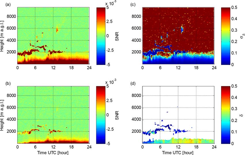
5810                                                                       V. Vakkari et al.: Aerosol particle depolarization ratio

                                                                        (e.g. Donovan et al., 2015). In Halo StreamLine lidars the in-
                                                                        strument telescope design has a matched field of view and di-
                                                                        vergence of 33 µrad (Table 1), and consequently the effect is
                                                                        small: in Fig. 2c δ ∗ increases by 0.0014 in 30 m. For instance,
                                                                        for the system modelled by Donovan et al. (2015) in-cloud
                                                                        multiple scattering increases the depolarization ratio from 0
                                                                        to 0.05 in approx. 50 m. Nevertheless, to minimize the effect
                                                                        of multiple scattering we only consider δ ∗ at the cloud base
                                                                        for the determination of the average bleed-through and use
                                                                        measurements in several clouds.
                                                                           For low-level clouds, we have observed saturation of the
Figure 2. Profiles at Limassol, Cyprus, on 2 May 2017 at                co-polar signal in the more powerful StreamLine XR instru-
12:08 UTC. (a) Co- and cross-polar SNR. A liquid cloud at ap-           ments. Signal saturation at liquid cloud base is readily identi-
prox. 800 m a.g.l. results in full attenuation of signal. Below cloud   fied as a non-linear relationship between co- and cross-polar
layer aerosol signal is visible. Above 1 km variability in SNR is due   SNR. For the measurement cases analysed here, we did not
to instrumental noise only. (b) The same as panel (a) but limited to    observe indications of saturation. Furthermore, we note that
lowest 1 km a.g.l. (c) Ratio of cross-polar SNR to co-polar SNR up      δ ∗ at cloud base should be determined with as high a time
to 1 km a.g.l. calculated from profiles in panel (a). Error bars rep-
                                                                        resolution as possible to ensure that both co- and cross-polar
resent uncertainty due to instrumental noise estimated from SNR at
                                                                        measurements represent the same part of the cloud. In prac-
>1 km a.g.l. in panel (a).
                                                                        tice, integration time is kept constant during a measurement
                                                                        campaign and was set as a compromise between temporal
                                                                        resolution and signal strength. We mitigate the effect of poor
level. Hence, the measured depolarization ratio can be safely           time resolution by choosing cases where cloud base remains
assumed to represent the particle linear depolarization ratio.          at the same altitude (within lidar resolution) for some tens of
   In Fig. 2a, consecutive co- and cross-polar SNR profiles             minutes and thus one can assume temporal homogeneity. No
are presented, where aerosol signal is observed up to 800 m             vertical smoothing is applied in calculating δ ∗ , as the signal
above ground level (a.g.l.) and a liquid cloud base is ob-              at cloud base is strong compared to the aerosol signal. Fi-
served at 840 m a.g.l. In liquid cloud the signal attenuates            nally, it should be noted that, especially in higher latitudes, it
quickly, and above 1 km the profiles represent instrumental             is not always trivial to find purely liquid phase clouds. Typi-
noise only. We use the measurements above 1 km to calculate             cally, mixed-phase clouds can be distinguished by the depo-
standard deviations of co-polar SNR (σco ) and cross-polar              larizing features of ice crystals. That is, in the histogram of
SNR (σcross ). In Fig. 2c, the raw depolarization ratio (δ ∗ )          δ ∗ at cloud base a secondary peak with higher δ ∗ than liquid
is calculated simply as the ratio of cross-polar SNR to co-             clouds would occur, which was not the case for our study.
polar SNR, and uncertainty is estimated from σco and σcross                To characterize the Halo polarizer bleed-through, we de-
by Gaussian error propagation.                                          termined the δ ∗ at liquid cloud base during both campaigns
   The construction of Halo StreamLine lidars does not in-              (Fig. 3). During the campaign at Limassol, we determined
clude a calibrator for depolarization channel, unlike PollyXT           δ ∗ at cloud base on 25 April and on 2 May 2017. From the
lidars for instance (Engelmann et al., 2016). Furthermore, the          distribution in Fig. 3a, the bleed-through is 0.011 ± 0.007
user cannot change the optical path to include a calibrator or          (mean ± standard deviation). At Vehmasmäki, we utilized
check the depolarizing effects of the individual components.            clouds on 13, 14 and 16 May 2016 as shown in Fig. 3b. At
Therefore, we are limited to evaluating the Halo depolariza-            Vehmasmäki, the estimated bleed-through is 0.016 ± 0.009
tion ratio at liquid cloud base.                                        (mean ± standard deviation). The mean cloud base δ ∗ val-
   Spherical cloud droplets do not polarize the directly                ues observed for these two systems in Fig. 3 are well in line
backscattered radiation, and thus non-zero δ ∗ at liquid cloud          with our experience with these and five other StreamLine and
base is an indication of incomplete extinction (or bleed-               StreamLine XR systems in Finland, where cloud base δ ∗ typ-
through) in the lidar internal polarizer. However, measure-             ically ranges from 0.01 to 0.02.
ment of δ ∗ at cloud base can be biased by signal saturation               We attribute the spread in the distributions in Fig. 3 mostly
or changes in cloud properties between co- and cross-polar              to variability of the clouds at the measurement sites and to the
measurement. Furthermore, multiple scattering results in in-            fact that co- and cross-polar measurements are consecutive
creasing depolarization signal inside a liquid cloud (e.g. Liou         and not simultaneous. Given that the cross-polar measure-
and Schotland, 1971). This increase in in-cloud δ ∗ is clearly          ment channel is constructed with fibre-optic technology, we
seen in Fig. 2c: at cloud base δ ∗ is 0.0102, and at the next           do not expect changes in the performance of the polarizer.
gate 30 m deeper inside the cloud δ ∗ has increased to 0.0116.          This is also our experience with Halo systems in Finland
   The magnitude of the multiple scattering effect on depo-             since 2016, but we recommend to check the bleed-through
larization ratio depends on both cloud and lidar properties             monthly or after an instrument is moved to a new location.

Atmos. Chem. Phys., 21, 5807–5820, 2021                                                   https://doi.org/10.5194/acp-21-5807-2021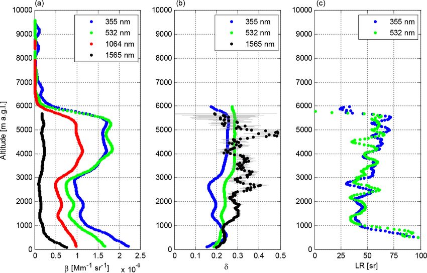
V. Vakkari et al.: Aerosol particle depolarization ratio                                                                         5811

                                                                      at 532 nm (Bohlmann et al., 2019). Due to the biaxial con-
                                                                      struction of emission and detection units, complete overlap
                                                                      is reached at 800–900 m a.g.l. (Engelmann, et al., 2016), and
                                                                      thus only measurements >800 m a.g.l. are utilized for this
                                                                      study (Bohlmann et al., 2019). The original spatial resolu-
                                                                      tion is 30 m and temporal resolution 30 s for the Vehmasmäki
                                                                      system (Bohlmann et al., 2019).
                                                                         At Limassol, PollyXT operated the same receiver chan-
                                                                      nels as the Vehmasmäki system had and additionally a cross-
Figure 3. Ratio of cross-polar SNR to co-polar SNR at liquid cloud    polar channel at 355 nm, together with a near-range telescope
base measured with Halo Doppler lidar. (a) Distribution of cloud      with 355 and 532 nm receiver channels. The near-range chan-
base δ ∗ at Limassol. (b) Distribution of cloud base δ ∗ at Vehmas-
                                                                      nels enable retrieval of optical properties down to 150 m a.g.l.
mäki.
                                                                      (Engelmann et al., 2016). Raw spatial resolution is 7.5 m and
                                                                      temporal resolution is 30 s.
Considering the large natural variability of the depolarization          During night-time, the Raman method (Ansmann et al.,
ratio (e.g. Illingworth et al., 2015; Baars et al., 2016) we find     1992) is used to retrieve aerosol optical properties from
the spread of observations in Fig. 3 tolerable. The standard          the raw signals. For daytime measurements, the method of
deviation in Fig. 3 is included in the uncertainty calculation        Klett (1981) can be utilized. Here, we present only mea-
of the Halo depolarization ratio.                                     surements when the Raman method was applied. The cal-
   We account for the observed bleed-through (B) in calcu-            ibration of the depolarization ratio was performed at both
lating Halo particle linear depolarization ratio (δ1565 ) as          Vehmasmäki and Limassol using the so-called 190◦ method
                                                                      (Freudenthaler, 2016), and the relative uncertainty in the par-
      SNRcross − B · SNRco                                            ticle linear depolarization ratio was estimated to be 10 %.
δ=                         ,                                   (2)
             SNRco
                                                                      2.3     Auxiliary data
where SNRco and SNRcross are the observed co- and cross-
polar SNR, respectively. Uncertainty in SNRcross corrected            Air mass history was estimated with the Hybrid Single-
for bleed-through (i.e. numerator in Eq. 2) is estimated as           Particle Lagrangian Integrated Trajectory model, HYSPLIT
           v                                                          (Stein et al., 2015). HYSPLIT was run through the READY
                                                                      website (Rolph et al., 2017) using the NCEP Global Data
                                                     !
                                        2
           u                                      2
           u                          σB        σco
               2
σcross,B = tσcross + (B · SNRco )2 ·      +           ,     (3)       Assimilation System (GDAS) meteorology at 0.5◦ horizontal
                                      B 2 SNR2co                      resolution. Back trajectories of 96 h arriving at the elevation
                                                                      of aerosol layers of interest were calculated.
where σB is standard deviation of the distribution in Fig. 3.
Finally, uncertainty in δ1565 taking into account instrumental
noise and uncertainty in bleed-through is estimated as                3     Results
         v
         u             2
                     σcross,B                2                        In this section we analyse observations of dust, marine and
         u                                  σco
σδ = |δ| t                             +        .          (4)        pollen aerosols during the Limassol and Vehmasmäki cam-
           (SNRcross − B · SNRco )2 SNR2co                            paigns, where said aerosol types were observed simulta-
                                                                      neously with Halo and PollyXT lidars. Dust and marine
2.2    PollyXT                                                        aerosols were observed during the Limassol campaign in the
                                                                      eastern Mediterranean, and pollen was observed during the
PollyXT is a multiwavelength Raman lidar capable of de-               Vehmasmäki campaign in a boreal forest region in Finland.
polarization ratio measurement at one or two wavelengths              We conclude this section with an overall comparison of the
depending on instrument configuration (Baars et al., 2016;            depolarization ratio measurements with the two instruments.
Engelmann et al., 2016). PollyXT emits simultaneously 355,
532 and 1064 nm wavelength pulses at a repetition frequency           3.1     Elevated dust layers
of 20 Hz. All PollyXT lidars are built with the same de-
sign, but there are small differences in the number of receiver       3.1.1    Limassol 21 April 2017
channels equipped in each individual system. A detailed de-
scription of PollyXT design is given by Baars et al. (2016)           Right at the beginning of Halo measurements at Limassol
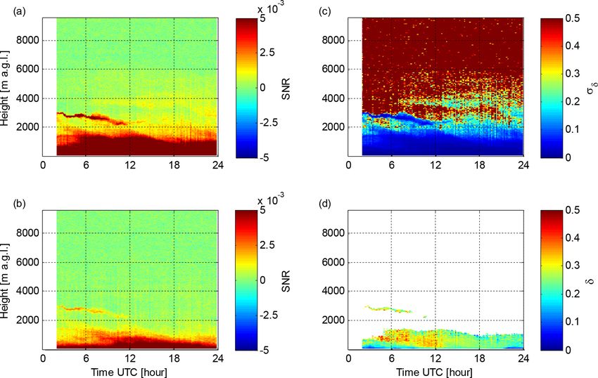
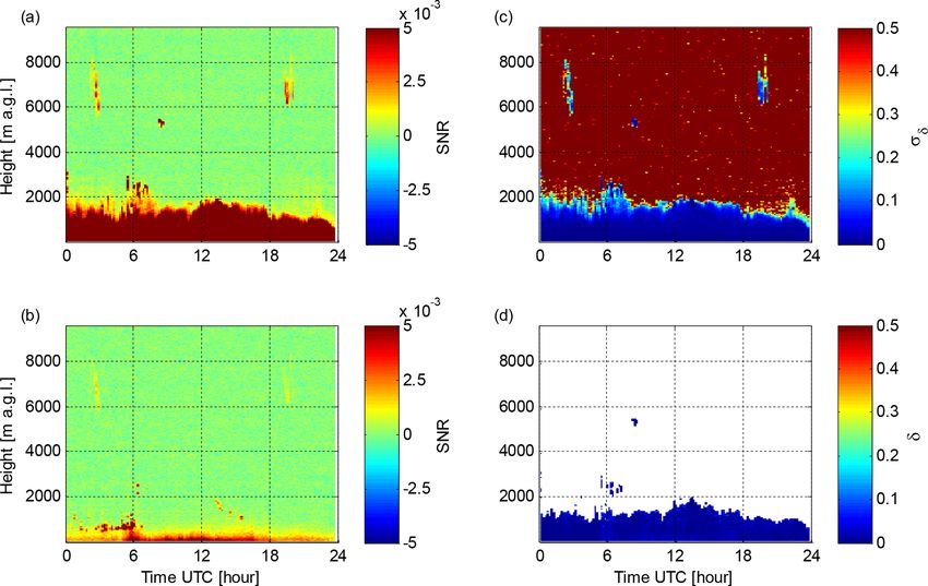
and Engelmann et al. (2016).                                          on 21 April 2017, several elevated layers were observed as
   At Vehmasmäki, PollyXT was configured with elastic                 seen in Fig. 4. Although Halo can observe elevated layers up
backscatter channels (355, 532 and 1064 nm); Raman-shifted            to 6 km a.g.l. on this day, the signal is too weak to retrieve
channels at 387, 407 and 607 nm; and a cross-polar channel            their depolarization ratio. This is clearly visible in the uncer-

https://doi.org/10.5194/acp-21-5807-2021                                                Atmos. Chem. Phys., 21, 5807–5820, 2021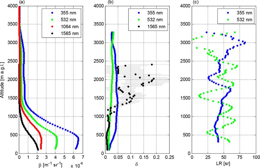
5812                                                                        V. Vakkari et al.: Aerosol particle depolarization ratio

Figure 4. Limassol 21 April 2017 measurements with Halo Doppler          Figure 5. Averaged profiles at Limassol on 21 April 2017 at 20:00–
lidar. (a) Time series of co-polar SNR at 300 s integration time.        21:30 UTC. All profiles have been smoothed by a 300 m running
(b) Time series of cross-polar SNR at 300 s integration time. (c) Un-    mean. (a) Backscatter by PollyXT (wavelengths 355–1064 nm) and
certainty in the depolarization ratio. (d) Particle linear depolariza-   attenuated backscatter by Halo (1565 nm). (b) Particle linear de-
tion ratio filtered with σδ
V. Vakkari et al.: Aerosol particle depolarization ratio                                                                                 5813

Figure 7. Limassol 27 April 2017 measurements with Halo Doppler
                                                                         Figure 9. Back trajectories of 96 h arriving at Limassol on 27 April.
lidar. (a) Time series of co-polar SNR at 300 s integration time.
                                                                         Back trajectories arriving at 19:00 and 02:00 UTC are included.
(b) Time series of cross-polar SNR at 300 s integration time. (c) Un-
certainty in the depolarization ratio. (d) Particle linear depolariza-
tion ratio filtered with σδ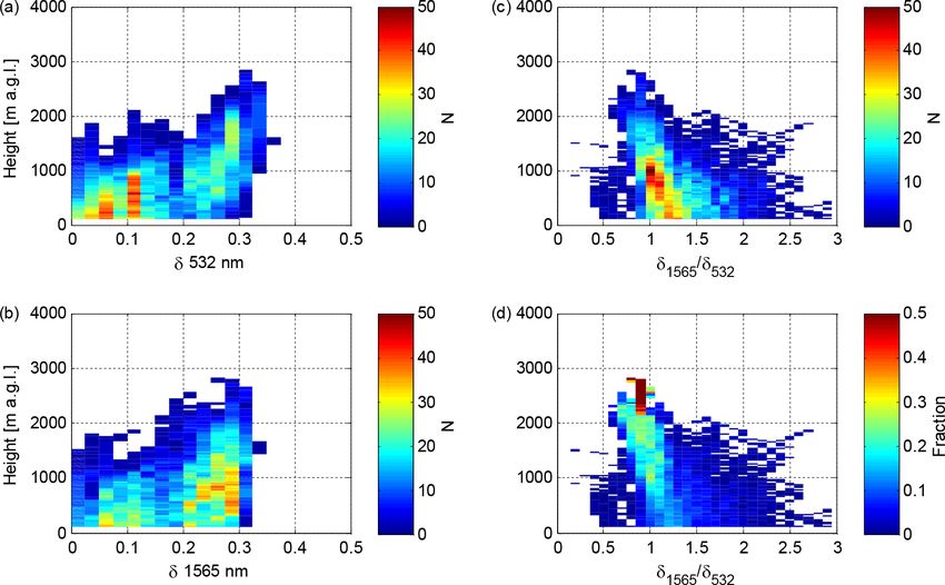
5814                                                                      V. Vakkari et al.: Aerosol particle depolarization ratio

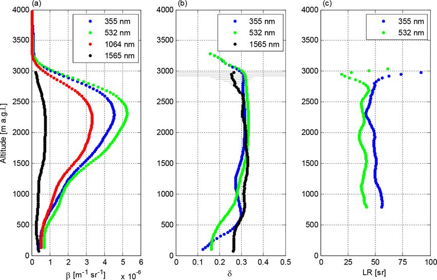
Figure 11. Averaged profiles at Limassol on 20 May 2017 at 19:55–      Figure 13. Vehmasmäki 15 May 2016 measurements with Halo
21:30 UTC. All profiles have been smoothed by a 300 m running          Doppler lidar. (a) Time series of co-polar SNR at 350 s integration
mean. (a) Backscatter by PollyXT (wavelengths 355–1064 nm) and         time. (b) Time series of cross-polar SNR at 350 s integration time.
attenuated backscatter by Halo (1565 nm). (b) Particle linear de-      (c) Uncertainty in the depolarization ratio. (d) Particle linear depo-
polarization ratio. Error bars represent measurement uncertainty.      larization ratio filtered with σδ
V. Vakkari et al.: Aerosol particle depolarization ratio                                                                          5815

                                                                        effects. For instance, any bias in the estimated bleed-through
                                                                        in the Halo polarizer would show up as bias in Fig. 15a and
                                                                        b. However, such bias is not present in the cases when δ355
                                                                        and/or δ532 are low.
                                                                           Considering the sources at Limassol during the campaign,
                                                                        the higher δ1565 for intermediate depolarization ratios rang-
                                                                        ing from 0.1 to 0.25 likely represents mixtures of dust with
                                                                        other aerosol types. A mixture of coarse, polarizing dust
                                                                        with less polarizing and smaller aerosol would result in the
                                                                        observed spectral dependency of the depolarization ratio.
                                                                        For aged-dust-dominated cases, lower depolarization ratios
                                                                        at longer wavelength could be due to the faster removal of
                                                                        coarse particles compared to submicron aerosol (e.g. Bur-
                                                                        ton et al., 2015). In any case, the observed wavelength de-
Figure 15. Comparison of particle linear depolarization ratio at dif-
                                                                        pendency in Fig. 15a–c for large δ suggests that, for dust-
ferent wavelengths. Observations represent 30 m vertical resolution
and have been smoothed by a 300 m running mean. To reduce scat-         dominated cases, smaller particle sizes have, on average, a
ter, a stricter uncertainty threshold is applied, and only data for     higher depolarization ratio at Limassol.
σδ 0.2. However, above about
eraged to match the temporal resolution of PollyXT Raman                1.5–2 km a.g.l., almost all retrievals indicate dust or dusty
retrievals (ranging from 45 min to 2 h).                                mixtures. Note that the vertical extent of the data is limited
   In Fig. 15a, three regions can be observed in the scat-              by the sensitivity of the Halo instrument, as Fig. 16a and b
terplot. For δ532 0.3, δ1565 is            and 532 nm exhibits a clear height dependency. Above about
lower than the depolarization ratio at the shorter wavelength.          1.5 km a.g.l., the majority of the observations present a lower
A very similar pattern is present in Fig. 15b: for δ355 0.3, δ1565 is lower     wavelength. In previous studies (Freudenthaler et al., 2009;
than δ355 . Similar regions appear even when comparing the              Groß et al., 2011; Burton et al., 2015; Haarig et al., 2017), a
two shorter wavelengths (Fig. 15c): for δ355 0.3, δ532 is lower than δ355 .                                probably mineral, dust for sub-1.5 km aerosols most of the
   Figure 15a–c also show similar correlations between the              time at Limassol.
depolarization ratios at different wavelengths. Therefore,
bearing in mind the similar patterns in all three scatterplots in
Fig. 15a–c, we consider the scatter to originate mainly from
the atmospheric aerosol properties rather than in instrumental

https://doi.org/10.5194/acp-21-5807-2021                                                 Atmos. Chem. Phys., 21, 5807–5820, 2021
5816 V. Vakkari et al.: Aerosol particle depolarization ratio
Figure 17. Particle linear depolarization ratio as a function of wave-
length for dust observations in Table 2. Additionally, spectral de-
pendency modelled with MOPSMAP based on the OPAC database
Figure 16. 2D histograms of the particle linear depolarization ratio for desert dust (Koepke et al., 2015; Gasteiger and Wiegner, 2018)
and height at Limassol using 30 m vertical resolution smoothed by a and AERONET inversion by Toledano et al. (2019) are included.
300 m running mean. Only data for σδ 0.20 at short wavelengths to δV. Vakkari et al.: Aerosol particle depolarization ratio 5817
Table 2. Spectral dependency of depolarization ratio for dust, marine aerosol and pollen.
Depolarization ratio
Time and origin 355 nm 532 nm 710 nm 1064 nm 1565 nm
This study, Limassol 21 Apr 2017 20:00–21:30; 0.19 ± 0.008 0.23 ± 0.008 0.29 ± 0.008
Saharan dust
27 Apr 2017 01:25–02:33; 0.36 ± 0.01 0.34 ± 0.002 0.30 ± 0.005
dust (Egypt)
27 Apr 2017 at 19:00– 0.31 ± 0.006 0.33 ± 0.005 0.32 ± 0.008
20:00;
dust (Turkey)
Haarig et al. (2017) Barbados 2013, 2014; 0.252 ± 0.030 0.280 ± 0.020 0.225 ± 0.022
Saharan dust
Burton et al. (2015) US 2014; Saharan dust 0.209 ± 0.015 0.304 ± 0.005 0.270 ± 0.005
Mexico Chihuahua 2013; 0.225 ± 0.041 0.373 ± 0.014 0.383 ± 0.006
local dust
Groß et al. (2011) Cabo Verde 2008; 0.24–0.27 0.29–0.31 0.36–0.40
Saharan dust
Freudenthaler et al. (2009) Morocco 2006; 0.24–0.28 0.31 ± 0.03 0.26–0.30 0.27 ± 0.04
Saharan dust
This study, Limassol 20 May 2017 at 19:55– 0.03 ± 0.01 0.015 ± 0.002 0.009 ± 0.003
21:30;
polluted marine
Groß et al. (2011) Cabo Verde 2008; marine 0.02 ± 0.01 0.02 ± 0.02
This study, Vehmasmäki 15 May 2016 19:00–21:00; 0.236 ± 0.009 0.269 ± 0.005
spruce and birch pollen
ization ratio at a wavelength of 1565 nm. Using observations at 1565 nm with a small decrease with increasing wave-
at liquid cloud base we have been able to characterize the length. The spruce and birch pollen depolarization ratio has
Halo Doppler lidar polarizer bleed-through with sufficient been characterized only recently at 532 nm (Bohlmann et al.,
accuracy to obtain useful depolarization ratio measurements; 2019). Our measurements indicate a slightly higher depolar-
uncertainty in the bleed-through is propagated to the depo- ization ratio of 0.27 at 1565 nm compared to 0.24 at 532 nm.
larization ratio measurement. A comparison of two different Overall, our results indicate that Halo Doppler lidars can add
Halo Doppler lidar systems with two PollyXT systems dur- another wavelength at 1565 nm to studies on the spectral de-
ing collocated measurements at Limassol, Cyprus, and Kuo- pendency of the particle linear depolarization ratio, at least
pio – Vehmasmäki, Finland, shows good agreement between in the lowest 2–3 km above ground.
the lidar systems. The agreement between the instruments For aerosol typing, adding a particle linear depolarization
is remarkably good considering the large wavelength differ- ratio at 1565 nm to shorter wavelengths can help to distin-
ence: the PollyXT depolarization ratio is retrieved at 355 guish biomass burning aerosols from dust, as a much stronger
and/or 532 nm. However, given the much lower laser energy spectral dependency has been observed for elevated biomass
in Halo Doppler lidars, it is not surprising that the vertical burning aerosols than for dust (e.g. Haarig et al., 2017, 2018;
extent of the usable depolarization ratio is much lower than Hu et al., 2019). In case there is prior knowledge of prevail-
for PollyXT. ing aerosols, such as transport of volcanic ash, even stand-
For relatively fresh mineral dust, we find particle lin- alone particle linear depolarization ratio measurements with
ear depolarization ratios at 1565 nm ranging from 0.29 to Halo Doppler lidars can probably provide useful information
0.32, which is in good agreement with previous observa- for aerosol typing.
tions, including measurements at the 710 and 1064 nm wave-
lengths (Freudenthaler et al., 2009; Groß et al., 2011; Bur-
ton et al., 2015; Haarig et al., 2017). For polluted marine Data availability. Processed lidar data are available upon request
aerosol we observed a very low depolarization ratio of 0.009 from the authors. Level 0 PollyXT observations are available
at https://polly.tropos.de/ (Polly NET, 2020, last access: 18 Au-
https://doi.org/10.5194/acp-21-5807-2021 Atmos. Chem. Phys., 21, 5807–5820, 20215818 V. Vakkari et al.: Aerosol particle depolarization ratio
gust 2020). Trajectory model HYSPLIT and GDAS meteorologi- Ansmann, A., Petzold, A., Kandler, K., Tegen, I., Wendisch,
cal data are available at https://www.ready.noaa.gov/HYSPLIT.php M., Mueller, D., Weinzierl, B., Mueller, T., and Heintzen-
(ARL, 2020, last access: 18 August 2020). berg, J.: Saharan Mineral Dust Experiments SAMUM-1 and
SAMUM-2: what have we learned?, Tellus B, 63, 403–429,
https://doi.org/10.1111/j.1600-0889.2011.00555.x, 2011.
Author contributions. Conceptualization and formal analysis were Ansmann, A., Mamouri, R.-E., Bühl, J., Seifert, P., Engelmann, R.,
carried out by VV, while investigation was carried out by HB, SB, Hofer, J., Nisantzi, A., Atkinson, J. D., Kanji, Z. A., Sierau,
JB, MK, RM and EJO’C. Data curation was carried out by VV, B., Vrekoussis, M., and Sciare, J.: Ice-nucleating particle ver-
HB, SB, MK and EJO’C. VV wrote the original draft, which was sus ice crystal number concentration in altocumulus and cirrus
reviewed and edited by VV, HB, SB, MK and EJO’C. layers embedded in Saharan dust: a closure study, Atmos. Chem.
Phys., 19, 15087–15115, https://doi.org/10.5194/acp-19-15087-
2019, 2019.
Competing interests. The authors declare that they have no conflict ARL: HYSPLIT-WEB, available at: https://www.ready.noaa.gov/
of interest. HYSPLIT.php, last access: 18 August 2020.
Baars, H., Kanitz, T., Engelmann, R., Althausen, D., Heese,
B., Komppula, M., Preißler, J., Tesche, M., Ansmann, A.,
Wandinger, U., Lim, J.-H., Ahn, J. Y., Stachlewska, I. S.,
Special issue statement. This article is part of the special issue
Amiridis, V., Marinou, E., Seifert, P., Hofer, J., Skupin, A.,
“Tropospheric profiling (ISTP11) (AMT/ACP inter-journal SI)”. It
Schneider, F., Bohlmann, S., Foth, A., Bley, S., Pfüller, A., Gian-
is a result of the 11th edition of the International Symposium on
nakaki, E., Lihavainen, H., Viisanen, Y., Hooda, R. K., Pereira,
Tropospheric Profiling (ISTP), Toulouse, France, 20–24 May 2019.
S. N., Bortoli, D., Wagner, F., Mattis, I., Janicka, L., Markowicz,
K. M., Achtert, P., Artaxo, P., Pauliquevis, T., Souza, R. A. F.,
Sharma, V. P., van Zyl, P. G., Beukes, J. P., Sun, J., Rohwer, E.
Acknowledgements. The authors gratefully acknowledge the G., Deng, R., Mamouri, R.-E., and Zamorano, F.: An overview of
NOAA Air Resources Laboratory (ARL) for the provision of the the first decade of PollyNET: an emerging network of automated
HYSPLIT transport and dispersion model and READY website Raman-polarization lidars for continuous aerosol profiling, At-
(https://www.ready.noaa.gov, last access: 18 August 2020) used in mos. Chem. Phys., 16, 5111–5137, https://doi.org/10.5194/acp-
this publication. 16-5111-2016, 2016.
Baars, H., Seifert, P., Engelmann, R., and Wandinger, U.:
Target categorization of aerosol and clouds by continu-
Financial support. This research has been supported by the Na- ous multiwavelength-polarization lidar measurements, Atmos.
tional Emergency Supply Agency of Finland. The Vehmasmäki Meas. Tech., 10, 3175–3201, https://doi.org/10.5194/amt-10-
pollen study and data evaluation have been supported by the 3175-2017, 2017.
Academy of Finland (grant no. 310312). The Limassol, Cyprus, Bohlmann, S., Shang, X., Giannakaki, E., Filioglou, M., Saarto,
observations have been supported by the SIROCCO project (grant A., Romakkaniemi, S., and Komppula, M.: Detection and char-
no. EXCELLENCE/1216/0217) co-funded by the Republic of acterization of birch pollen in the atmosphere using a mul-
Cyprus and the structural funds of the European Union for Cyprus tiwavelength Raman polarization lidar and Hirst-type pollen
through the Research and Innovation Foundation and EXCELSIOR sampler in Finland, Atmos. Chem. Phys., 19, 14559–14569,
project that received funding from the European Union (H2020- https://doi.org/10.5194/acp-19-14559-2019, 2019.
WIDESPREAD-04-2017: Teaming Phase 2) project under grant Burton, S. P., Ferrare, R. A., Hostetler, C. A., Hair, J. W., Rogers, R.
agreement no. 857510 and from the Republic of Cyprus. R., Obland, M. D., Butler, C. F., Cook, A. L., Harper, D. B., and
Froyd, K. D.: Aerosol classification using airborne High Spectral
Resolution Lidar measurements – methodology and examples,
Review statement. This paper was edited by Andreas Richter and Atmos. Meas. Tech., 5, 73–98, https://doi.org/10.5194/amt-5-73-
reviewed by two anonymous referees. 2012, 2012.
Burton, S. P., Hair, J. W., Kahnert, M., Ferrare, R. A., Hostetler,
C. A., Cook, A. L., Harper, D. B., Berkoff, T. A., Seaman, S.
T., Collins, J. E., Fenn, M. A., and Rogers, R. R.: Observa-
References tions of the spectral dependence of linear particle depolariza-
tion ratio of aerosols using NASA Langley airborne High Spec-
Achtert, P., Brooks, I. M., Brooks, B. J., Moat, B. I., Prytherch, tral Resolution Lidar, Atmos. Chem. Phys., 15, 13453–13473,
J., Persson, P. O. G., and Tjernström, M.: Measurement of wind https://doi.org/10.5194/acp-15-13453-2015, 2015.
profiles by motion-stabilised ship-borne Doppler lidar, Atmos. COESA: U.S. Standard Atmosphere, 1976, U.S. Government Print-
Meas. Tech., 8, 4993–5007, https://doi.org/10.5194/amt-8-4993- ing Office, Washington, DC, 227 pp., 1976.
2015, 2015. Donovan, D. P., Klein Baltink, H., Henzing, J. S., de Roode, S.
Ansmann, A., Wandinger, U., Riebesell, M., Weitkamp, C., and R., and Siebesma, A. P.: A depolarisation lidar-based method
Michaelis, W.: Independent measurement of extinction and for the determination of liquid-cloud microphysical properties,
backscatter profiles in cirrus clouds by using a combined Atmos. Meas. Tech., 8, 237–266, https://doi.org/10.5194/amt-8-
Raman elastic-backscatter lidar, Appl. Opt., 31, 7113–7131, 237-2015, 2015.
https://doi.org/10.1364/AO.31.007113, 1992.
Atmos. Chem. Phys., 21, 5807–5820, 2021 https://doi.org/10.5194/acp-21-5807-2021V. Vakkari et al.: Aerosol particle depolarization ratio 5819 Engelmann, R., Kanitz, T., Baars, H., Heese, B., Althausen, D., Plu, M., Robertson, L., Rokitansky, C.-H., Scherllin-Pirscher, Skupin, A., Wandinger, U., Komppula, M., Stachlewska, I. S., B., Sievers, K., Sofiev, M., Som de Cerff, W., Steinheimer, Amiridis, V., Marinou, E., Mattis, I., Linné, H., and Ansmann, M., Stuefer, M., Theys, N., Uppstu, A., Wagenaar, S., Win- A.: The automated multiwavelength Raman polarization and kler, R., Wotawa, G., Zobl, F., and Zopp, R.: A volcanic-hazard water-vapor lidar PollyXT: the neXT generation, Atmos. Meas. demonstration exercise to assess and mitigate the impacts of vol- Tech., 9, 1767–1784, https://doi.org/10.5194/amt-9-1767-2016, canic ash clouds on civil and military aviation, Nat. Hazards 2016. Earth Syst. Sci., 20, 1719–1739, https://doi.org/10.5194/nhess- Frehlich, R. G. and Kavaya, M. J.: Coherent laser radar perfor- 20-1719-2020, 2020. mance for general atmospheric refractive turbulence, Appl. Opt., Hu, Q., Goloub, P., Veselovskii, I., Bravo-Aranda, J.-A., Popovici, 30, 5325–5352, https://doi.org/10.1364/AO.30.005325, 1991. I. E., Podvin, T., Haeffelin, M., Lopatin, A., Dubovik, O., Freudenthaler, V.: About the effects of polarising optics on lidar Pietras, C., Huang, X., Torres, B., and Chen, C.: Long-range- signals and the 190 calibration, Atmos. Meas. Tech., 9, 4181– transported Canadian smoke plumes in the lower stratosphere 4255, https://doi.org/10.5194/amt-9-4181-2016, 2016. over northern France, Atmos. Chem. Phys., 19, 1173–1193, Freudenthaler, V., Esselborn, M., Wiegner, M., Heese, B., Tesche, https://doi.org/10.5194/acp-19-1173-2019, 2019. M., Ansmann, A., MüLLER, D., Althausen, D., Wirth, M., Illingworth, A. J., Barker, H. W., Beljaars, A., Ceccaldi, M., Fix, A., Ehret, G., Knippertz, P., Toledano, C., Gasteiger, J., Chepfer, H., Clerbaux, N., Cole, J., Delanoë, J., Domenech, Garhammer, M., and Seefeldner, M.: Depolarization ratio profil- C., Donovan, D. P., Fukuda, S., Hirakata, M., Hogan, R. J., ing at several wavelengths in pure Saharan dust during SAMUM Huenerbein, A., Kollias, P., Kubota, T., Nakajima, T., Naka- 2006, Tellus B, 61, 165–179, https://doi.org/10.1111/j.1600- jima, T. Y., Nishizawa, T., Ohno, Y., Okamoto, H., Oki, R., 0889.2008.00396.x, 2009. Sato, K., Satoh, M., Shephard, M. W., Velázquez-Blázquez, A., Gasteiger, J. and Wiegner, M.: MOPSMAP v1.0: a versatile Wandinger, U., Wehr, T., and van Zadelhoff, G.-J.: The Earth- tool for the modeling of aerosol optical properties, Geosci. CARE Satellite: The Next Step Forward in Global Measurements Model Dev., 11, 2739–2762, https://doi.org/10.5194/gmd-11- of Clouds, Aerosols, Precipitation, and Radiation, Bull. Am. Me- 2739-2018, 2018. teorol. Soc., 96, 1311–1332, https://doi.org/10.1175/BAMS-D- Gialitaki, A., Tsekeri, A., Amiridis, V., Ceolato, R., Paulien, L., 12-00227.1, 2015. Kampouri, A., Gkikas, A., Solomos, S., Marinou, E., Haarig, M., IPCC: Climate Change 2013: The Physical Science Basis. Contri- Baars, H., Ansmann, A., Lapyonok, T., Lopatin, A., Dubovik, O., bution of Working Group I to the Fifth Assessment Report of the Groß, S., Wirth, M., Tsichla, M., Tsikoudi, I., and Balis, D.: Is the Intergovernmental Panel on Climate Change, Cambridge Uni- near-spherical shape the “new black” for smoke?, Atmos. Chem. versity Press, Cambridge, United Kingdom and New York, NY, Phys., 20, 14005–14021, https://doi.org/10.5194/acp-20-14005- USA, available at: http://www.climatechange2013.org (last ac- 2020, 2020. cess: 10 August 2020), 2013. Groß, S., Tesche, M., Freudenthaler, V., Toledano, C., Wiegner, M., Klett, J. D.: Stable analytical inversion solution for Ansmann, A., Althausen, D., and Seefeldner, M.: Characteriza- processing lidar returns, Appl. Opt., 20, 211–220, tion of Saharan dust, marine aerosols and mixtures of biomass- https://doi.org/10.1364/AO.20.000211, 1981. burning aerosols and dust by means of multi-wavelength Koepke, P., Gasteiger, J., and Hess, M.: Technical Note: Optical depolarization and Raman lidar measurements during SA- properties of desert aerosol with non-spherical mineral parti- MUM 2, Tellus B, 63, 706–724, https://doi.org/10.1111/j.1600- cles: data incorporated to OPAC, Atmos. Chem. Phys., 15, 5947– 0889.2011.00556.x, 2011. 5956, https://doi.org/10.5194/acp-15-5947-2015, 2015. Groß, S., Freudenthaler, V., Wiegner, M., Gasteiger, J., Geiß, A., Liou, K.-N. and Schotland, R. M.: Multiple Backscattering and and Schnell, F.: Dual-wavelength linear depolarization ratio of Depolarization from Water Clouds for a Pulsed Lidar Sys- volcanic aerosols: Lidar measurements of the Eyjafjallajökull tem, J. Atmos. Sci., 28, 772–784, https://doi.org/10.1175/1520- plume over Maisach, Germany, Atmos. Environ., 48, 85–96, 0469(1971)0282.0.CO;2, 1971. https://doi.org/10.1016/j.atmosenv.2011.06.017, 2012. Mamouri, R.-E. and Ansmann, A.: Potential of polariza- Haarig, M., Ansmann, A., Althausen, D., Klepel, A., Groß, S., tion lidar to provide profiles of CCN- and INP-relevant Freudenthaler, V., Toledano, C., Mamouri, R.-E., Farrell, D. A., aerosol parameters, Atmos. Chem. Phys., 16, 5905–5931, Prescod, D. A., Marinou, E., Burton, S. P., Gasteiger, J., En- https://doi.org/10.5194/acp-16-5905-2016, 2016. gelmann, R., and Baars, H.: Triple-wavelength depolarization- Mamouri, R.-E. and Ansmann, A.: Potential of polarization/Raman ratio profiling of Saharan dust over Barbados during SALTRACE lidar to separate fine dust, coarse dust, maritime, and anthro- in 2013 and 2014, Atmos. Chem. Phys., 17, 10767–10794, pogenic aerosol profiles, Atmos. Meas. Tech., 10, 3403–3427, https://doi.org/10.5194/acp-17-10767-2017, 2017. https://doi.org/10.5194/amt-10-3403-2017, 2017. Haarig, M., Ansmann, A., Baars, H., Jimenez, C., Veselovskii, Manninen, A. J., O’Connor, E. J., Vakkari, V., and Petäjä, T.: A gen- I., Engelmann, R., and Althausen, D.: Depolarization and eralised background correction algorithm for a Halo Doppler li- lidar ratios at 355, 532, and 1064 nm and microphysi- dar and its application to data from Finland, Atmos. Meas. Tech., cal properties of aged tropospheric and stratospheric Cana- 9, 817–827, https://doi.org/10.5194/amt-9-817-2016, 2016. dian wildfire smoke, Atmos. Chem. Phys., 18, 11847–11861, Manninen, A. J., Marke, T., Tuononen, M., and O’Connor, https://doi.org/10.5194/acp-18-11847-2018, 2018. E. J.: Atmospheric Boundary Layer Classification With Hirtl, M., Arnold, D., Baro, R., Brenot, H., Coltelli, M., Eschbacher, Doppler Lidar, J. Geophys. Res.-Atmos., 123, 8172–8189, K., Hard-Stremayer, H., Lipok, F., Maurer, C., Meinhard, D., https://doi.org/10.1029/2017JD028169, 2018. Mona, L., Mulder, M. D., Papagiannopoulos, N., Pernsteiner, M., https://doi.org/10.5194/acp-21-5807-2021 Atmos. Chem. Phys., 21, 5807–5820, 2021
5820                                                                         V. Vakkari et al.: Aerosol particle depolarization ratio

Papagiannopoulos, N., Mona, L., Amodeo, A., D’Amico, G., Gumà             Stein, A. F., Draxler, R. R., Rolph, G. D., Stunder, B. J. B., Co-
  Claramunt, P., Pappalardo, G., Alados-Arboledas, L., Guerrero-             hen, M. D., and Ngan, F.: NOAA’s HYSPLIT Atmospheric
  Rascado, J. L., Amiridis, V., Kokkalis, P., Apituley, A., Baars, H.,       Transport and Dispersion Modeling System, Bull. Am. Meteo-
  Schwarz, A., Wandinger, U., Binietoglou, I., Nicolae, D., Bortoli,         rol. Soc., 96, 2059–2077, https://doi.org/10.1175/BAMS-D-14-
  D., Comerón, A., Rodríguez-Gómez, A., Sicard, M., Papayannis,              00110.1, 2015.
  A., and Wiegner, M.: An automatic observation-based aerosol             Toledano, C., Torres, B., Velasco-Merino, C., Althausen, D., Groß,
  typing method for EARLINET, Atmos. Chem. Phys., 18, 15879–                 S., Wiegner, M., Weinzierl, B., Gasteiger, J., Ansmann, A.,
  15901, https://doi.org/10.5194/acp-18-15879-2018, 2018.                    González, R., Mateos, D., Farrel, D., Müller, T., Haarig, M.,
Päschke, E., Leinweber, R., and Lehmann, V.: An assessment of the            and Cachorro, V. E.: Sun photometer retrievals of Saharan dust
  performance of a 1.5 µm Doppler lidar for operational vertical             properties over Barbados during SALTRACE, Atmos. Chem.
  wind profiling based on a 1-year trial, Atmos. Meas. Tech., 8,             Phys., 19, 14571–14583, https://doi.org/10.5194/acp-19-14571-
  2251–2266, https://doi.org/10.5194/amt-8-2251-2015, 2015.                  2019, 2019.
Pearson, G., Davies, F., and Collier, C.: An Analysis of the Per-         Tuononen, M., O’Connor, E. J., Sinclair, V. A., and Vakkari,
  formance of the UFAM Pulsed Doppler Lidar for Observing                    V.: Low-Level Jets over Utö, Finland, Based on Doppler Li-
  the Boundary Layer, J. Atmos. Ocean. Technol., 26, 240–250,                dar Observations, J. Appl. Meteor. Climatol., 56, 2577–2594,
  https://doi.org/10.1175/2008JTECHA1128.1, 2009.                            https://doi.org/10.1175/JAMC-D-16-0411.1, 2017.
Pentikäinen, P., O’Connor, E. J., Manninen, A. J., and Ortiz-             Vakkari, V., O’Connor, E. J., Nisantzi, A., Mamouri, R. E., and Had-
  Amezcua, P.: Methodology for deriving the telescope focus func-            jimitsis, D. G.: Low-level mixing height detection in coastal lo-
  tion and its uncertainty for a heterodyne pulsed Doppler lidar, At-        cations with a scanning Doppler lidar, Atmos. Meas. Tech., 8,
  mos. Meas. Tech., 13, 2849–2863, https://doi.org/10.5194/amt-              1875–1885, https://doi.org/10.5194/amt-8-1875-2015, 2015.
  13-2849-2020, 2020.                                                     Vakkari, V., Manninen, A. J., O’Connor, E. J., Schween, J. H.,
Polly NET: Worldwide observations with the portable Raman lidar              van Zyl, P. G., and Marinou, E.: A novel post-processing algo-
  systems (Polly), available at: https://polly.tropos.de/, last access:      rithm for Halo Doppler lidars, Atmos. Meas. Tech., 12, 839–852,
  18 August 2020.                                                            https://doi.org/10.5194/amt-12-839-2019, 2019.
Rolph, G., Stein, A., and Stunder, B.: Real-time Environmental Ap-
  plications and Display sYstem: READY, Environ. Model. Softw.,
  95, 210–228, https://doi.org/10.1016/j.envsoft.2017.06.025,
  2017.

Atmos. Chem. Phys., 21, 5807–5820, 2021                                                      https://doi.org/10.5194/acp-21-5807-2021
You can also read


