Are Bitcoin Bubbles Predictable? Combining a Generalized Metcalfe's Law and the LPPLS Model
←
→
Page content transcription
If your browser does not render page correctly, please read the page content below
Are Bitcoin Bubbles Predictable?
                                             Combining a Generalized Metcalfe’s Law and the LPPLS Model
arXiv:1803.05663v1 [econ.EM] 15 Mar 2018

                                           Spencer Wheatley1∗ , Didier Sornette1,2∗ , Tobias Huber1 , Max Reppen3 , and Robert N. Gantner
                                                       1
                                                           ETH Zurich, Department of Management, Technology and Economics, Switzerland
                                                                  2
                                                                      Swiss Finance Institute, c/o University of Geneva, Switzerland
                                                                              3
                                                                                  ETH Zurich, Department of Mathematics
                                                                            e-mails: swheatley@ethz.ch, dsornette@ethz.ch
                                                                                         ∗
                                                                                             corresponding authors

                                                                                          March 16, 2018

                                                                                                Abstract

                                                  We develop a strong diagnostic for bubbles and crashes in bitcoin, by analyzing the coincidence
                                              (and its absence) of fundamental and technical indicators. Using a generalized Metcalfe’s law based
                                              on network properties, a fundamental value is quantified and shown to be heavily exceeded, on
                                              at least four occasions, by bubbles that grow and burst. In these bubbles, we detect a universal
                                              super-exponential unsustainable growth. We model this universal pattern with the Log-Periodic
                                              Power Law Singularity (LPPLS) model, which parsimoniously captures diverse positive feedback
                                              phenomena, such as herding and imitation. The LPPLS model is shown to provide an ex-ante
                                              warning of market instabilities, quantifying a high crash hazard and probabilistic bracket of the crash
                                              time consistent with the actual corrections; although, as always, the precise time and trigger (which
                                              straw breaks the camel’s back) being exogenous and unpredictable. Looking forward, our analysis
                                              identifies a substantial but not unprecedented overvaluation in the price of bitcoin, suggesting many
                                              months of volatile sideways bitcoin prices ahead (from the time of writing, March 2018).

                                                                                                    1
1 Introduction
In 2008, pseudonymous Satoshi Nakamoto introduced the digital decentralized cryptocurrency,
bitcoin [1], and the innovative blockchain technology that underlies its peer-to-peer global payment
network1 . Since its techno-libertarian beginnings, which envisioned bitcoin as an alternative to the
central banking system, bitcoin has experienced super-exponential growth. Fueled by the rise of bit-
coin, a myriad of other cryptocurrencies have erupted into the mainstream with a range of highly
disruptive use-cases foreseen. Cryptocurrencies have become an emerging asset class [3]. At the end
of 2017, the price of bitcoin peaked at almost 20’000 USD, and the combined market capitalization of
cryptocurrencies reached around 800 billion USD.
The explosive growth of bitcoin intensified debates about the cryptocurrency’s intrinsic or funda-
mental value. While many pundits have claimed that bitcoin is a scam and its value will eventually
fall to zero, others believe that further enormous growth and adoption await, often comparing to the
market capitalization of monetary assets, or stores of value. By comparing bitcoin to gold, an analogy
that is based on the digital scarcity that is built into the bitcoin protocol, some markets analysts pre-
dicted bitcoin prices as a high as 10 million per bitcoin [4]. Nobel laureate and bubble expert, Robert
Shiller, epitomized this ambiguity of bitcoin price predictions when he stated, at the 2018 Davos World
Economic Forum, that “bitcoin could be here for 100 years but it’s more likely to totally collapse” and,
“you just put an upper bound on [bitcoin] with the value of the world’s money supply. But that upper
bound is awfully big. So it can be anywhere between zero and there.” [5].
There is an emerging academic literature on cryptocurrency valuations [6, 7, 8, 9, 10, 11, 12, 13, 14]
and their growth mechanisms [15]. Many of these studies attribute some technical feature of the
bitcoin protocol, such as the “proof-of-work” system on which the bitcoin cryptocurrency is based, as
a source of value2 . However, as has been proposed by former Wall Street analyst Tom Lee [4], an early
academic proposal (see Ref.[17]), by now widely discussed within cryptocurrency communities, is that
an alternative valuation of bitcoin can be based on its network of users. In the 1980s, Metcalfe proposed
that the value of a network is proportional to the square of the number of nodes [18]. This may also
be called the network effect, and has been found to hold for many networked systems. If Metcalfe’s
law holds here, fundamental valuation of bitcoin may in fact be far easier than valuation of equities
3 —which relies on various multiples, such as price-to-earnings, price-to-book, or price-to-cash-flow
ratios—and will therefore admit an indication of bubbles.
Although it seems relatively obvious that bubbles exist within cryptocurrencies, it is not a straw
1
In this network, transactions, which do not rely on an intermediary, are verified by network nodes and, through
cryptography, immutably recorded in a decentralized publicly distributed ledger [2].
2
The question of what constitutes the value of money has preoccupied generations of thinkers. About 2050 years ago,
Aristotle was probably the first to argue that money needed a high cost of production in order to make it valuable. In
other words, according to Aristotle, the larger the effort to create new money, the more valuable it is. This was later
elaborated into the labor theory of value, starting with Adam Smith, David Ricardo, and becoming the central thesis
of Marxian economics. Nowadays, this concept is archaic and it is well understood that money is credit (see e.g., [16]).
It is thus puzzling that cryptocurrencies with proof-of-work designs, which aim at revolutionizing money and exchanges
between individuals, use a very old and obsolete concept that has been mostly abandoned in economics.
3
See however Cauwels and Sornette [19, 20], who developed an original valuation method for social network firms
based on the economic value of the demographics of users, and were able to predict ex-ante the performance of companies
such as Facebook, Zynga and Groupon after their IPO’s.
2man argument that, in finance and economics, financial bubbles are often excluded based on market
efficiency rationalization4 , which assume an unpredictable market price, for instance following a kind
of geometrical random walk (see e.g., [22]). In sharp contrast, Didier Sornette and co-workers claim
that bubbles exist and are ubiquitous. Moreover, they can be accurately described by a deterministic
nonlinear trend called the Log-Periodic Power Law Singularity (LPPLS) model, potentially with highly
persistent, but ultimately mean-reverting, errors. The LPPLS model combines two well documented
empirical and phenomenological features of bubbles (see [23] for a recent review):
1. the price exhibits a transient faster-than-exponential growth (i.e., where the growth rate itself is
growing)—resulting from positive feedbacks like herding [24]—that is modeled by a hyperbolic
power law with a singularity in finite time, i.e., endogenously approaching an infinite value and
therefore necessitating a crash or correction before the singularity is reached;
2. it is also decorated with accelerating log-periodic volatility fluctuations, embodying spirals of
competing expectations of higher returns (bullish) and an impending crash (bearish) [25, 26].
Such log-periodic fluctuations are ubiquitous in complex systems with a hierarchical structure
and also appear spontaneously as a result of the interplay between (i) inertia, (ii) nonlinear
positive and (iii) nonlinear negative feedback loops [27].
The model thus characterizes a process in which, as speculative frenzy intensifies, the bubble
matures towards its endogenous critical point, and becomes increasingly unstable, such that any small
disturbance can trigger a crash. This has been further formalized in the so-called JLS model where
the rate of return accelerates towards a singularity, compensated by the growing crash hazard rate
[25, 28], providing a generalized return-risk relationship. We emphasize that one should not focus on
the instantaneous and rather unpredictable trigger itself, but monitor the increasingly unstable state
of the bubbly market, and prepare for a correction.
Here, we combine—as a fundamental measure—a generalized Metcalfe’s law and—as a technical
measure—the LPPLS model, in order to diagnose bubbles in bitcoin. When both measures coincide,
this provides a convincing indication of a bubble and impending correction. If, in hindsight, such
signals are followed by a correction similar to that suggested, they provide compelling evidence that a
bubble and crash did indeed take place.
This paper is organized as follows. In the first part, we document a generalized Metcalfe’s law
describing the growth of the population of active bitcoin users. We show that the generalized Metcalfe’s
law provides a support level, and that the ratio of market capitalization to “the Metcalfe value” gives
a relative valuation ratio. On this basis, we identify a current substantial but not unprecedented
overvaluation in the price of bitcoin. In the second part of the paper, we unearth a universal super-
exponential bubble signature in four bitcoin bubbles, which corresponds to the LPPLS model with a
reasonable range of parameters. The LPPLS model is shown to provide advance warning, in particular
with confidence intervals for the critical bursting time based on profile likelihood. An LPPLS fitting
algorithm is presented, allowing for selection of the bubble start time, and offering an interval for the
crash time, in a probabilistically sound way. We conclude the paper with a brief discussion.
4
For instance, the Efficient Market Hypothesis (EMH) assumes that prices quasi-instantaneously reflects all available
information. Thus, market crashes result from novel very negative information that gets incorporated into prices [21].
32 Fundamental value of bitcoin: active users & a generalized Met-
calfe’s law
Metcalfe’s law states that the value, in this case market capitalization (cap), of a network is,
p = eα0 uβ0 , β0 = 2, (1)
where u is called the number of active users, imperfectly quantified by a proxy, being the number of
active addresses5 . It is a single factor model for a fundamental valuation of bitcoin, and plausibly
for other cryptocurrencies. From Figure 1, we indeed see a surprisingly clear log-linear relationship.
Rather than taking Metcalfe’s law as a given, we estimate the relevant parameters by a log-linear
regression model, which we refer to as the (generalized) Metcalfe law,
ln(p) = α + β ln(u) + ǫ. (2)
The result of this fit, on 2’782 daily values, from 17-07-2010 to 26-02-2018, is a slope β = 1.69
(standard error 0.0076), intercept α = 1.51 (0.087), and coefficient of determination R2 = 0.956 .
Forcing the exponent β to be equal to 2 would result in an intercept of −2.01 (0.018), but this
regression is significantly worse than the above7 . Further, a slope of 2 (or larger) is robustly rejected
on moving windows8 . On this basis, it seems that the value 2 proposed by Metcalfe is too large, at
least for the bitcoin ecosystem.9
It should be noted that this regression severely violates the assumption that the errors be inde-
pendent and identically distributed, as there are persistent deviations from the regression line. This
statement deserves to be made in more salient terms: the residuals are in fact the bubbles and crashes!
This is the focus of the second part of this paper. Ignoring this egregious violation of the so-called
Gauss–Markov conditions is well known to give the false impression of precise parameter estimates.
Further, endogeneity is an issue, as the number of active users may determine market cap in the long
term, but large fluctuations in market cap can also plausibly trigger fluctuations in active users on
shorter time scales (see Figure 1). We address this by smoothing active users10 , assuming that this will
5
The data is collected from bitinfocharts.com. Limitations: It is difficult to know the true number of active users, in
particular because a single user can have multiple addresses that, to an outsider, cannot be distinguished from addresses
belonging to multiple users. Moreover, bitcoin.org’s Developer Guide [29] discourages key reuse, advising that each key
should only be used for two transactions (to receive, then send), and that all change should be sent to a new address,
generated at the time of transaction (belonging to the sender). Depending on to what extent this advice is followed, this
measure is thus an unclear mix between the number of daily users and the number of daily transactions (their activity).
6
Such high values are of limited value as one often obtains high coefficients of determination when regressing unrelated
trending/non-stationary series onto each-other (so-called “spurious regression”). In this case, the causal link between
active users and market cap is assumed.
7
An ANOVA/F-test comparing the two models gives a p-value of less than 10−16 . Further, the calibrated value of the
slope, β = 1.69, with standard error 0.0076, is clearly far from Metcalfe’s value 2.
8
On 83% of 1-year windows, the parameter β is less than 2, and on 75% of windows the parameter β is significantly
less than 2, at level p = 0.05.
9
Note, however, that the measure of u is overestimating the true number of daily users. It is possible that this does
affect the precise value of the exponent β. On the other hand, it could provide an underestimate of the number of active
users if the typical user does not transact daily.
10
This is done with the R library loess with 5 equivalent degrees of freedom.
4Figure 1: Left panel: Scatterplot of the bitcoin market cap versus the number of active users, with
logarithmic scales. The points becomes darker as time progresses, and the three latest crashes are
indicated by colored points, and arrows indicating the size of the correction. The generalized Metcalfe
regression is given in solid red, and with slope forced to be 2 given by the dashed red line. Right panel:
Active users (rough black line), again in a logarithmic scale, as a function of time, with linear scale
inset. A scaled bitcoin market cap is overlaid with the grey line. The red and dashed yellow lines are
the nonlinear regression fits of active users, fitting on different time windows.
average out the effects of short term feedback of market cap onto active users. A multiplier effect is
also a plausible consequence of this endogeneity: a jump in user activity causes an increment in market
cap, which triggers a (smaller) jump in user activity, feeding back into market cap, etc. Therefore, we
do not claim to isolate the effect of a single increment in active users on market cap, and do not need
it. Finally, we omit formal tests for causality, given the plausibility of the general mechanism behind
Metcalfe’s law, as well as the very turbulent and only long-term adherence to it11 .
In view of these limitations, the generalized Metcalfe’s law here is still rather impressive, and
will be shown to be highly useful, despite its radical simplicity and uncertain parameter values. Of
course, one may add other variables to the regression, which further characterize the network, such as
degree of centralization, transaction costs, volume, etc. However, the actual volume (value of authentic
transactions) for instance is not only difficult to know, but, in general financial markets, is known to
be highly correlated with volatility, of which bubbles and bursts are the most formidable contributors,
and may therefore be too endogenous to soundly indicate a fundamental value. Therefore, the variable
‘active users’ is retained as the focal quantity.
Looking at Figure 1, a clear and important feature is the shrinking growth rate of active users
11
The exponent value 2 in the standard Metcalfe’s law embodies the idea that the value of the network is proportional
to the total number of interactions or exchanges, which themselves scales as the total number of possible connections. In
other words, Metcalfe’s law assumes full connectivity between all users. This does not seem realistic. Our finding of a
smaller exponent β ≈ 1 + 2/3 expresses a more sparsely connected network in which each user is on average linked to
∼ N 2/3 other users in the total network of N users. For instance, for N=1 Million, a typical user is then connected to
“only” 10’000 other users, a more realistic figure.
5which we model by a relatively flexible ecological-type nonlinear regression,
d
ln(u) = a − be−ct + ǫ, (3)
which saturates at a “carrying capacity”, u → ea as t → ∞, and where the log transform stabilizes the
noise level. As in the case of the generalized Metcalfe regression, here there is clear structure in the
residuals, as feedback loops develop between the number of active users and price during speculative
bubbles. We opt to fit the curve (3) by OLS (ordinary least squares) and treat it as a rough estimate:
Fitting from 2012-01-01 to 2018-02-2612 , the annual growth rate is expected to decrease over the next
five years from 35% to 21%, taking the expected level of active users from 0.79 Million currently to 2.60
Million in 2023 with 5% and 8% standard errors, respectively. Comparing with a fit starting earlier, in
2010-10-2413 , again a similarly decreasing growth rate is confirmed, but with predictions for 2018 and
2023 respectively being 7% and 28% larger than predictions for the first fit. More generally, within the
sample, the fitted curves are similar, but, beyond the sample, differences explode such that there are
4 orders of magnitude difference between the predicted carrying capacities. Here, model uncertainty
dominates uncertainty of estimated parameters. There is also likely to be some non-stationarity and
regime-shifts as the bitcoin network evolves and matures, contributing another level of uncertainty
in the long-term extrapolation of our models. Therefore, precise inference based on a single model—
notably omitting any limitation imposed by the physical bitcoin network—is misleading, and long-term
predictions effectively meaningless. However, smoothing of past values is not problematic, and short
term projections may be reasonable.
Given the number of active users, and calibrations of the generalized Metcalfe’s law, which maps
to market cap, we can now compare the predicted market cap with the true one, as in Figure 2. Also,
using smoothed active users, the local endogeneities—where price drives active users—are assumed
to be averaged out. The OLS estimated regression, by definition, fits the conditional mean, as is
apparent in Figure 2. Therefore, if bitcoin has evolved based on fundamental user growth with transient
overvaluations on top, then the OLS estimate will give an estimate in-between and thus above the
fundamental value. For this reason, support lines are also given, and—although their parameters are
chosen visually—they may give a sounder indication of fundamental value. In any case, the predicted
values for the market cap indicate a current over-valuation of at least four times. In particular, the
OLS fit with parameters (1.51,1.69), the support line with (0,1.75), and the Metcalfe support line (-3,2)
suggest current values around 44, 22, and 33 billion USD, respectively, in contrast to the actual current
market cap of 170 billion USD. Further, assuming continued user growth in line with the regression of
active users starting in 2012, the end of 2018 Metcalfe predictions for the market cap are 77, 39, and
12
Details of the fit: The interval spanned by the natural log of the number of active users was transformed to (0,1)
by shifting by 9.483 and dividing by 4.46. The time span was also transformed to (0,1). The nonlinear regression was
then fit by OLS, giving parameters and standard deviations a=1.72 (0.14), b= 1.76 (0.15), c=0.79 (0.09), d=0.70 (0.26).
Predicted values (transformed back to original scale) for the first day of each year from 2018–2023 in Millions of active
users, and percentage standard error are 0.788 (0.05%), 1.06 (0.06%), 1.39 (0.07%), 1.75 (0.07%), 2.16 (0.074%), and 2.60
(0.08%). Finally, the estimated carrying capacity is 2.76 × 10⁷ with standard error of 86%.
13
Doing the same as for the previous fit, but starting from 2010-10-24, gives parameters: a = 2.86 (0.59)b =
3.03 (0.61), c = 0.46 (0.11), d = 0.40 (0.02), with predicted values for first day of 2018–2023: 0.812, 1.14, 1.54, 2.04,
2.63, and 3.35 (Millions). The predicted growth rates over the next five years are 40%, 36%, 32%, 29%, and 27%. And a
massive carrying capacity of 9.39 × 10¹¹ is predicted with 180% standard error.
610
1010
Metcalfe Exponent on Window
Bitcoin Market Cap
5
108
0
106
-5
2012 2014 2016 2018
Figure 2: Comparing bitcoin market cap (black line) with predicted market cap based on various
generalized Metcalfe regressions of active users. The rough red line is given by plugging the true
number of active users into the generalized Metcalfe regression shown in Figure 1, having OLS estimated
coefficients (α, β) = (1.51, 1.69). The remaining lines plug smoothed active users (non-parametric up
to 2018 and the nonlinear regression starting in 2012 to project beyond) into the generalized Metcalfe
formula with different parameters: The smooth green line for the estimated coefficients (1.51,1.69); the
orange dashed line is proposed as a “support line”, having coefficients (0,1.75) specified by eye; the blue
dash-dotted line being a Metcalfe support line with coefficients (-3,2). The grey line, plotted against
the right axis, is the exponent of the generalized Metcalfe regression onto smoothed active users on
a causal 60 day moving window (i.e., window on the previous 60 days). It is truncated to emphasize
fluctuations around the value 2 (solid grey line).
64 billion USD respectively14 , which is still less than half of the current market cap. These results are
found to be robust with regards to the chosen fitting window15 .
On this basis alone, the current market looks similar to that of early 2014, which was followed by
a year of sideways and downward movement. Some separate fundamental development would need to
exist to justify such high valuation, which we are unaware of.
14
With standard errors already above 10% induced by estimated parameters, excluding additional prediction uncertainty
due to persistent fluctuations of active users about the mean.
15
Although the parameters vary depending on the fitting window, even allowing for fitting windows starting in 2016,
where one obtains a high exponent β (above 2.5), an overvaluation of about a factor of two is still indicated.
73 Bitcoin bubbles: universality of unsustainable growth?
3.1 Identification and main properties of the four main bubbles
Using the generalized Metcalfe regression onto smoothed active users as well as its support lines,
one can identify in Figure 2 four main bubbles corresponding to the largest upward deviations of the
market cap from this estimated fundamental value. These four bubbles in market cap are highlighted
in Figure 3, and detailed in Table 1—in some cases exhibiting a 20 fold increase in less than 6 months!
In all cases, the burst of the bubble is attributed to fundamental events, listed below, in particular for
the first three bubbles, which corrected rapidly at the time of the clearly relevant news. The fourth
and very recent bubble was much longer, and it is plausible that the main news there was really the
20’000 USD value of bitcoin, i.e., it finally collapsed under its own weight16 . Market participants often
lament that crashes are unforeseeable due to the unpredictability of bad news.
2014 2016 2018
18-12-17
1010
23-11-13
4
11-04-13 3
Normalized Log Mcap
Bitcion Market Cap
4
2
18-08-12
108
1
3
2
6
1
10
t0=0 tc=1
Figure 3: Upper triangle: market cap of bitcoin with four major bubbles indicated by bold colored
lines, numbered, and with bursting date given. Lower triangle: The four bubbles scaled to have the
same log-height and length, with the same color coding as the upper, and with pure hyperbolic power
law and LPPLS models fitted to the average of the four scaled bubbles, given in dashed and solid black,
respectively.
However, focusing on the news that may have triggered the crash is akin to waiting for “the
final straw”, rather than monitoring the developing unsustainable load on the poor camel’s back. Of
16
This large valuation is likely to have attracted “whales” to cash a part of their bitcoin portfolios, ei-
ther to realize their profit or due to operational constraints. For instance, it was revealed on March
2, 2018 that Nobuaki Kobayashi, bankruptcy trustee for Mt. Gox, once the largest bitcoin exchange
in the world, has sold off about $400 million in bitcoin and bitcoin cash since late September 2017
(https://www.zerohedge.com/news/2018-03-07/bitcoins-tokyo-whale-sells-400m-bitcoin-bitcoin-cash).
8Bubble Start End Days M-Cap0 M-Cap1 Growth Mean Return
1 2012-05-25 2012-08-18 84 4.65 × 10⁷ 1.45 × 10⁸ 3.1 0.013
2 2013-01-03 2013-04-11 98 1.39 × 10⁸ 2.84 × 10⁹ 20.4 0.031
3 2013-10-07 2013-11-23 47 1.45 × 10⁹ 9.8 × 10⁹ 6.8 0.042
4 2015-06-08 2017-12-18 924 3.17 × 10⁹ 3.27 × 10¹¹ 103 0.005
5 2017-03-31 2017-12-18 155 1.69 × 10¹⁰ 3.27 × 10¹¹ 21 0.02
Table 1: Bubble statistics. Columns: Start, end (time of peak value, prior to correction), duration in
days, starting and peak market cap, growth factor (peak divided by start value: M-Cap1 / M-Cap0 ),
and average daily return. The bubbles correspond to the numbering in Figure 3. Bubble 5 corresponds
to approximately the last six months of the fourth bubble, and will be used in the next section. The
price data for bitcoin is from Bitstamp, in USD, hourly from 2012-01-01 to 2018-01-08; the bitcoin
circulating supply comes from blockchain.info.
particular interest here is that, although the height and length of the bubbles vary considerably, when
scaled to have the same log-height and length, a near-universal super-exponential growth is evident, as
diagnosed by the overall upward curvature in this linear-logarithmic plot (lower Figure 3). And in this
sense, like a sandpile, once the scaled bubble becomes steep enough (angle of repose), it will avalanche,
while the precise triggering nudge is essentially irrelevant.
Below, events thought to trigger crashes/corrections, corresponding to bubbles 1–4 in Table 1 are
mentioned17 :
0. 2011-06-1918 : Mt. Gox was hacked, causing the bitcoin price to fall 88% over the next 3 months.
1. 2012-08-28: Ponzi fraud of perhaps hundreds of thousands of bitcoin under the name bitcoins
Savings & Trust; charges filed by Securities and Exchange Commission.
2. 2013-04-10: Major bitcoin exchange, Mt Gox, breaks under high trading volume; price falls more
than 50% over next 2 days.
3. 2013-12-5: Following strong adoption growth in China, the People’s Bank of China bans financial
institutions from using bitcoin; bitcoin market cap drops 50% over the next two weeks. 07-02-
2014: operational issues at major exchanges due to distributed denial of service attacks, and two
weeks later Mt Gox closes.
4. 2017-12-28: South Korean regulator threatens to shut down crypto currency exchanges.
3.2 Log-periodic finite time singularity model
Following Sornette and colleagues [25, 28, 30], as mentioned in the introduction, we consider bubbles
to be the result of unsustainable (faster than exponential) growth, achieving an infinite return in finite
time (a finite time singularity), forcing a correction / change of regime in the real world. We adopt
the LPPLS model, as parameterized in [31], for the log market cap, pi at time ti ,
yi := ln(pi ) = a + (tc − ti )m b + c cos w ln(tc − ti ) + d sin w ln(tc − ti ) + ǫi , t i (4)
17
Events taken from https://99bitcoins.com/price-chart-history/
18
This trigger is for the “zeroth” bubble, being before our data window.
9where 0 < m < 1, ln(pc ) = a, and T1 ≤ ti < tc . T1 is the starting time, and tc the stopping or so-called
critical time by which the bubble must burst. This model combines two well documented empirical and
phenomenological features of bubbles: (1) a transient “faster-than-exponential” growth with singularity
at tc , modeled by a pure hyperbolic power law (the above equation with c = d = 0), resulting from
positive feedbacks, which is (2) decorated with accelerating periodic volatility fluctuations, embodying
spirals of fear and crash expectations.
The model needs to be fit with data ((y1 , t1 ), . . . , (yn , tn )), on a window (T1 , T2 ), where T1 ≤ t1 <
· · · < tn ≤ T2 < tc . The window (T1 , T2 ) needs to be specified, with selection of the start of the bubble
T1 often being less obvious. As is typical in time series regression [32], the errors ǫi are correlated and
may have changing variance (hetero-skedasticity), which if ignored leads to sub-optimal estimates, and
confidence intervals that are too small (over-optimistic). In this case, generalized least squares (GLS)
provides a conventional solution, which has been used with LPPLS [33, 34, 35] and, if well-specified,
has optimal properties. Here, we opt for a simple specification of the error model, being auto-regressive
of order 119 ,
ǫi = φǫi−1 + ηi , |φ| < 1, (5)
to model the rather persistent deviations from the overall trend. We then estimate the LPPLS model
by profiling over non-linear parameters (m, w, tc , φ), which allows the conditionally linear parameters
(a, b, c, d) to be estimated analytically, by GLS, or by OLS if φ = 0. Assuming white noise normal errors
ηi , this is maximum likelihood, and allows for profile likelihood confidence intervals of all parameters.
Here, we focus on tc , the critical time at which the bubble is most likely to burst. Before taking the
Metcalfe fundamental value into account, and to provide a curve to compare with the data in Figure 3,
we fit the pure hyperbolic power law (obtained by putting c = d = 0 in (4)) and the LPPLS model to
the average of the four scaled bubbles20 , with results summarized in Table 2. The hyperbolic power
law and LPPLS fits provide a similar trend, and the forward-looking predicted critical/bursting time
hugs the lower bound of 1.01 (the true peak being by construction at 1).
Perhaps curiously—despite fitting on an average of unsynchronized disparate bubbles with similar
overall trajectories—the LPPLS fit is significantly better, based on log-likelihood (p < 10−5 ) as it
captures some of the persistent fluctuations, and allows for a significantly smaller φ, i.e. a reduction
of the memory time ∼ 1/(1 − φ) of the residuals by a factor 1321 .
19
Higher order ARMA models can also be considered, and are seen to leave residuals with little auto-correlation. Given
the regression based de-trending, truly long memory in the errors is not expected, and the auto-correlation of residuals is
seen to decay clearly faster than a power law. Further, Dickey-Fuller tests tend to reject that the residuals are unit-root,
strongly when significant log periodic oscillations are fit.
20
These fits contain future information, in the sense that the end time of each fitted bubble is the time at which the
price peaked, which can only be determined after the crash occurred. These fits are thus not for prediction purpose but
for assessing the quality of the hyperbolic power law versus LPPLS models.
21
This suggests the existence of an intrinsic phase of the log-periodic oscillations with respect to the finite-time rounding
of the mathematical singularity at the market peak before the crash [36, 37].
10a b c d ω m tc φ
2.00 -1.97 -0.020 0.013 10.79 0.23 1.03(1.01,1.06) 0.87
1.54 -1.52 =0 =0 NA 0.31 1.02(1.01,1.05) 0.99
Table 2: LPPLS (second row) and pure hyperbolic power law (c = d = 0) (third row) fits on the
average of the four scaled bubbles shown in Figure 3. The sample is taken at 200 equidistant points.
The 95% profile likelihood confidence interval is given for tc .
3.3 Bubbles in the Market-to-Metcalfe Ratio
Given our proposed fundamental value of bitcoin based on the generalized Metcalfe regressions
presented above, we define the Market-to-Metcalfe value (MMV) ratio,
pi
MMVi = , (6)
e u2i
−3
as the actual market cap (pi at time ti ) divided by the market cap predicted by the Metcalfe support
level, with parameters (α0 = −3, β0 = 2) in (1), with smoothed active users (ui ) plugged in22 . We
sample the value every three hours over the time periods corresponding to bubbles 1–3 and 5 in Table
1.
As shown in Figure 4, bubbles are persistent deviations of the Market-to-Metcalfe value above
support level 1, which are well modelled by the LPPLS model. In particular, the parameters of the
hyperbolic power law and LPPLS models fitted on the Market-to-Metcalfe ratio data, for the full bubble
lengths, are given in Table 4. For the different bubbles, the key nonlinear parameters fall within similar
ranges, and calibration of tc is accurate. Again, the LPPLS fits dominate the pure hyperbolic power
laws, according to likelihood ratios. Further, based on our methodology (see appendix), none of these
fits can be rejected on the basis of their residuals.
22
Note that whether the value β = 2 or β = 1.75 are used, the results for this analysis will be effectively identical.
11et to Met atio Normalized
2
10
1
1
0
2012 2014 2016 2018 0 1
Figure 4: Left panel: Market-to-Metcalfe value ratio (MMV) over time. The apparent bubbles, which
radically depart from the fundamental level 1, are colored and given in Table 1 as bubbles 1–3 and
5. Right panel: for the same four bubbles, the MMV ratios are shown in log-scale as a function of
linear rescaled time, with 0.25 vertical offset for visibility. The hyperbolic power law and LPPLS fits
on the 4 full bubbles are shown. Values of the MMV ratio after the bubble peak are shown on the grey
background, where the colored vertical lines indicate the upper limit for tc of the 95% profile likelihood
confidence interval for each of the four bubbles. The three thin vertical black lines gives the rightmost
edge of the 95, 97.5, and 100% data windows on which fits were done, with parameters summarized in
Table 3 and Appendix Table 5.
The ex-ante predictive aspect is important as, in addition to verifying the LPPLS bubble in hind-
sight, one would like to have a sound advance warning of the bubble’s existence and a reasonable
confidence interval for its bursting time. Here, we provide a simple indication of this potential with
two additional sets of fits: fitting with bubble data up to 95% and 97.5% of the bubble length. The
overall parameter estimates (see appendix Table 6) are similar to the 100% window, in Table 4, with
key nonlinear parameters typically in ranges 0.1 < m < 0.5, and 7 < w < 11. Focusing on the criti-
cal bursting time, in Table 3, the estimated tc and 95% confidence intervals are given, showing quite
stable advance-warning. That is, point estimates and confidence intervals are consistent with the true
bursting time, noting that tc is in theory both the most probable and latest time for the burst of the
bubble [25, 28, 30], as the market is increasingly susceptible as it approaches tc , and can therefore be
toppled by bad news.
12Fit a b c d w m tc φ
1 2.74 -2.72 -0.051 -0.044 8.37 0.10 1.02 (1.01,1.09) 0.92
2 3.74 -3.73 -0.005 0.012 10.80 0.10 1.05 (1.03,1.06) 0.90
3 4.56 -4.53 -0.031 -0.013 8.97 0.10 1.09 (1.05,1.12) 0.92
5 1.09 -0.96 -0.071 0.053 12.00 0.38 1.01 (1.01,1.07) 0.98
1a 2.71 -2.68 =0 =0 NA 0.10 1.02 (1.01,1.04) 0.98
2a 2.13 -2.13 =0 =0 NA 0.18 1.04 (1.02,1.04) 0.99
3a 4.61 -4.59 =0 =0 NA 0.10 1.09 (1.05,1.23) 0.97
5a 1.046 -0.94 =0 =0 NA 0.43 1.00 (1.01,1.20) 0.99
Table 3: Estimated parameters of the LPPLS and hyperbolic power law models on the Market-to-
Metcalfe value ratios for the four bubbles, indicated by the fit number. The suffix ‘a’ corresponds to
the hyperbolic power law fits of the Market-to-Metcalfe value ratios for these four bubbles. The 95%
profile likelihood confidence interval for tc is given. The likelihood ratio test of the LPPLS versus the
hyperbolic power law (null) gives p-values of 0.01, 10−5 , 0.02, and 0.07, for these four bubbles. A lower
bound for m of 0.1 was enforced.
Fit 0.95 0.975 1
1 0.99 (0.98,1.08) 1.01 (0.99,1.08) 1.02 (1.01,1.09)
2 0.99 (0.98,1.0) 1.07 (1.05,1.07) 1.05 (1.03,1.06)
3 1.02 (1.01,1.02) 1.07 (1.04,1.08) 1.09 (1.05,1.12)
5 0.97 (0.97,0.98) 0.98 (1.01,1.06) 1.00 (1.01,1.07)
1a 0.99 (0.97,1.4) 1.01 (0.98,1.32) 1.02 (1.01,1.04)
2a 1.00 (0.99,1.04) 1.06 (1.04,1.11) 1.04 (1.02,1.04)
3a 1.08 (1.0,1.4) 1.08 (1.01,1.25) 1.09 (1.05,1.23)
5a 0.95 (0.95,1.4) 0.98 (0.98,1.4) 1.00 (1.01,1.20)
Table 4: Estimated critical time and 95% confidence interval, for LPPLS and hyperbolic power law
fits of the Market-to-Metcalfe value ratios of the four bubbles, indicated by the fit number and suffixed
with a, as defined in Table 3. The three columns are for fits on data up to T2 , being 95, 97.5, and
100% of the bubble length, as indicated by bubbles 1–3 and 5 in Table 1.
4 Discussion
In this paper, we have combined a generalized Metcalfe’s law, providing a fundamental value based
on network characteristics, with the Log-periodic Power law Singularity (LPPLS) model, to develop
a rich diagnostic of bubbles and their crashes that have punctuated the cryptocurrency’s history. In
doing so, we were able to diagnose four distinct bubbles, being periods of high overvaluation and
LPPLS-like trajectories, which were followed by crashes or strong corrections. Although the height
and length of the bubbles vary substantially, we showed that, when scaled to the same log-height and
length, a near-universal super-exponential growth is documented. This is in radical contrast to the
view that crypto-markets follow a random walk and are essentially unpredictable.
Further, in addition to being able to identify bubbles in hindsight, given the consistent LPPLS
bubble characteristics and demonstrated advance warning potential, the LPPLS can be used to provide
ex-ante predictions. For instance, a reasonable confidence interval for the endogeneous critical time
13indicates a high hazard for correction in that neighborhood, as any minor event could topple the
unstable market. Of course, massive exogeneous shocks, although rare, could occur at any time, and
the LPPLS model can provide no warning there.
Focusing on the outlook for bitcoin, the active user data indicates a shrinking growth rate, which a
range of parameterizations of our generalized Metcalfe’s law translates into slowing growth in market
capitalization. Further, our Metcalfe-based analysis indicates current support levels for the bitcoin
market in the range of 22–44 billion USD, at least four times less than the current level. On this basis
alone, the current market resembles that of early 2014, which was followed by a year of sideways and
downward movement. Given the high correlation of cryptocurrencies, the short-term movements of
other cryptocurrencies are likely to be affected by corrections in bitcoin (and vice-versa), regardless of
their own relative valuations.
14References
[1] Satoshi Nakamoto. Bitcoin: A peer-to-peer electronic cash system. 2008.
[2] Andreas M Antonopoulos. Mastering Bitcoin: unlocking digital cryptocurrencies. O’Reilly Media,
Inc., 2014.
[3] Chris Burniske and Jack Tatar. Cryptoassets: The Innovative Investor’s Guide to Bitcoin and
Beyond. McGraw-Hill, 2018.
[4] Sara Silverstein. Analyst says 94% of bitcoin’s price move-
ment over the past 4 years can be explained by one equation.
http://uk.businessinsider.com/bitcoin-price-movement-explained-by-one-equation-fundstrat-tom-
2017. [Online; accessed 01-Jan-2018].
[5] Ryan Browne. Nobel prize-winning economist Robert Shiller thinks bitcoin is an “interesting exper-
iment”. https://www.cnbc.com/2018/01/26/robert-shiller-says-bitcoin-is-an-interesting-experime
2018. [Online; accessed 27-Jan-2018].
[6] Nikolay Gertchev. The moneyness of bitcoin. Mises Daily, Auburn: Ludwig von Mises Institute,
4, 2013.
[7] Cameron Harwick. Cryptocurrency and the problem of intermediation. The Independent Review,
20(4):569–588, 2016.
[8] Jan A Bergstra and Peter Weijland. Bitcoin: a money-like informational commodity. arXiv
preprint arXiv:1402.4778, 2014.
[9] David Yermack. Is bitcoin a real currency? an economic appraisal. In Handbook of digital currency,
pages 31–43. Elsevier, 2015.
[10] Torbjørn Bull Jenssen. Why bitcoins have value, and why governments are sceptical. Master’s
thesis, Department of Economics, University of Oslo, 2014.
[11] Marshall Van Alstyne. Why bitcoin has value. Communications of the ACM, 57(5):30–32, 2014.
[12] Jamal Bouoiyour and Refk Selmi. What does bitcoin look like? Annals of Economics & Finance,
16(2):449–492, 2015.
[13] Michal Polasik, Anna Iwona Piotrowska, Tomasz Piotr Wisniewski, Radoslaw Kotkowski, and
Geoffrey Lightfoot. Price fluctuations and the use of bitcoin: An empirical inquiry. International
Journal of Electronic Commerce, 20(1):9–49, 2015.
[14] Yiteng Zhang. Economics of competing crypto currencies: Monetary policy, miner reward and
historical evolution. Thesis for the MSc Degree in Financial Computing at University College
London,2014.
15[15] Ke Wu, Spencer Wheatley, and Didier Sornette. Classification of crypto-coins and tokens from the
dynamics of their power law capitalisation distributions. arXiv preprint arXiv:1803.03088, 2018.
[16] Susanne von der Becke and Didier Sornette. Should banks be banned from creating money? an
analysis from the perspective of hierarchical money. Journal of Economic Issues, 51(4):1019–1032,
2017.
[17] Ken Alabi. Digital blockchain networks appear to be following metcalfe’s law. Electronic Com-
merce Research and Applications, 24:23–29, 2017.
[18] Bob Metcalfe. Metcalfe’s law after 40 years of Ethernet. Computer, 46(12):26–31, 2013.
[19] Peter Cauwels and Didier Sornette. Quis pendit ipsa pretia: Facebook valuation and diagnostic of
a bubble based on nonlinear demographic dynamics. Journal of Portfolio Management, 38(2):56–
66, 2012.
[20] Zalán Forró, Peter Cauwels, and Didier Sornette. When games meet reality: is Zynga overvalued?
Journal of Investment Strategies, 1(3):119–145, 2012.
[21] Eugene F Fama. Efficient capital markets: A review of theory and empirical work. The journal
of Finance, 25(2):383–417, 1970.
[22] Burton Gordon Malkiel. A random walk down Wall Street: including a life-cycle guide to personal
investing. WW Norton & Company, 1999.
[23] Didier Sornette, Peter Cauwels, et al. Financial bubbles: Mechanisms and diagnostics. Review of
Behavioral Economics, 2(3):279–305, 2015.
[24] Didier Sornette. Why stock market crash, Princeton University Press, new preface. 2017.
[25] Anders Johansen, Didier Sornette, and Olivier Ledoit. Predicting financial crashes using discrete
scale invariance. Risk, 1(4):5–32, 1999.
[26] Didier Sornette. Discrete-scale invariance and complex dimensions. Physics Reports, 297(5):239–
270, 1998 (extended version at http://xxx.lanl.gov/abs/cond-mat/9707012).
[27] Kayo Ide and Didier Sornette. Oscillatory finite-time singularities in finance, population and
rupture. Physica A: Statistical Mechanics and its Applications, 307(1-2):63–106, 2002.
[28] Anders Johansen, Olivier Ledoit, and Didier Sornette. Crashes as critical points. International
Journal of Theoretical and Applied Finance, 3(2):219–255, 2000.
[29] Bitcoin developer guide. https://bitcoin.org/en/developer-guide. [Online; accessed 12-Mar-
2018].
[30] Didier Sornette, Ryan Woodard, Wanfeng Yan, and Wei-Xing Zhou. Clarifications to questions
and criticisms on the Johansen-Ledoit-Sornette financial bubble model. Physica A: Statistical
Mechanics and its Applications, 392(19):4417–4428, 2013.
16[31] Vladimir Filimonov and Didier Sornette. A stable and robust calibration scheme of the log-periodic
power law model. Physica A: Statistical Mechanics and its Applications, 392(17):3698–3707, 2013.
[32] William H Greene. Econometric analysis (international edition). 2000.
[33] L Gazola, C Fernandes, A Pizzinga, and R Riera. The log-periodic-AR(1)-GARCH(1, 1) model
for financial crashes. The European Physical Journal B, 61(3):355–362, 2008.
[34] Li Lin, RE Ren, and Didier Sornette. The volatility-confined LPPL model: A consistent model
of “explosive” financial bubbles with mean-reverting residuals. International Review of Financial
Analysis, 33:210–225, 2014.
[35] Špela Jezernik Širca and Matjaž Omladič. The JLS model with ARMA/GARCH errors. Ars
Mathematica Contemporanea, 13(1):63–79, 2016.
[36] Anders Johansen and Didier Sornette. Evidence of discrete scale invariance by canonical averaging.
Int. J. Mod. Phys. C, 9(3):433–447, 1998.
[37] Wei-Xing Zhou and Didier Sornette. Non-parametric analyses of log-periodic precursors to finan-
cial crashes. Int. J. Mod. Phys. C, 14(8):1107–1126, 2003.
[38] José C Pinheiro and Douglas M Bates. Linear mixed-effects models: basic concepts and examples.
Mixed-effects models in S and S-Plus, pages 3–56, 2000.
175 Appendix
97.5%
Fit a b c d w m tc φ
1 2.72 -2.72 -0.035 -0.062 7.76 0.10 1.01 (0.99,1.08) 0.92
2 3.88 -3.87 -0.004 0.013 11.39 0.10 1.07 (1.05,1.07) 0.90
3 4.32 -4.30 -0.035 -0.012 8.37 0.10 1.07 (1.04,1.08) 0.92
5 0.91 -0.79 -0.062 0.074 11.34 0.48 0.98 (1.01,1.06) 0.98
1a 2.62 -2.60 =0 =0 NA 0.10 1.01 (0.98,1.32) 0.96
2a 3.88 -3.87 =0 =0 NA 0.10 1.06 (1.04,1.11) 0.98
3a 4.58 -4.56 =0 =0 NA 0.10 1.08 (1.01,1.25) 0.97
5a 0.86 -0.77 =0 =0 NA 0.58 0.98 (0.98,1.4) 0.99
95%
Fit a b c d w m tc φ
1 2.53 -2.52 -0.059 -0.040 7.76 0.10 0.99 (0.98,1.08) 0.92
2 1.42 -1.44 0.013 0.007 10.79 0.26 0.99 (0.98,1.0) 0.90
3 2.96 -2.95 -0.004 0.043 10.18 0.13 1.02 (1.01,1.02) 0.93
5 0.81 -0.71 -0.054 0.085 11.40 0.57 0.97 (0.97,0.98) 0.96
1a 2.47 -2.45 =0 =0 NA 0.10 0.99 (0.97,1.4) 0.96
2a 1.54 -1.55 =0 =0 NA 0.25 1.00 (0.99,1.04) 0.98
3a 4.60 -4.58 =0 =0 NA 0.10 1.08 (1.0,1.4) 0.96
5a 0.75 -0.68 =0 =0 NA 0.70 0.95 (0.95,1.4) 0.99
Table 5: The same as Table 3, but fits up to 95%, and 97.5% of the bubble length, rather than 100%.
The likelihood ratio test p-values of bubbles 1–3 and 5, with the pure hyperbolic power law fit as the
null, for the first sub-table are 0.05, 0. 0007, 0.01, and 0.02; and for the second sub-table, 0.05, < 10−6 ,
0.0004, and 0.003.
5.1 LPPLS algorithm
A rough algorithm for fitting LPPL is given, and illustrated with a data example in Figure 5.
Assumed are existence of a smooth trend in a window before the finite time singularity at tc , and that
a stationary time series model exists for the—often persistent—errors around that trend. It allows for
selection of a best window, giving the bubble starting time, T1 , by a hypothesis test, and confidence
intervals for the critical time tc , which are more realistic than if assuming iid errors.
Steps
1. Identify initial error model: Take broad window (T0 , T2 ) thought to contain the bubble, T0 <
T1 < T2 < tc . Fit the log market cap with a flexible non-parametric curve to obtain an estimate
of the trend. We use the R loess library and Akaike Information Criterion (AIC) to select
degrees of freedom. Then fit the error-model, here an AR(1) time series, onto the de-trended
data, giving an initial estimate for the GLS LPPLS estimation.
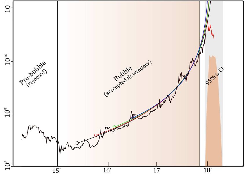
18Figure 5: 2015–2018 bitcoin market cap bubble to serve as an illustration for the algorithm. Plotted
are four accepted pure power law regressions, with upper limit of the fitting window T2 placed 2 months
prior to the turning point, and with four different values of the bubble starting time, T1 . The orange
mode is the average of the four profile likelihoods for tc for the four fits shown up to the 95% level,
bounded by the light grey bar, giving the 95% interval.
2. Characterize error variance: Bootstrap the residuals from step 1 and feed them through the fitted
AR(1) to simulate errors, allowing for the distribution of the residual standard error on different
window sizes to be approximated by Monte Carlo. Due to the autocorrelated errors, a chi-square
distribution will not be valid.
3. Fit LPPLS function by profile-likelihood with GLS: Given a fitting window (T1 , T2 ), take a fine
grid of nonlinear parameters (m, w, tc ), and for each point do a GLS fit with, in this case AR(1)
errors, initialized from step 1. A maximum likelihood implementation of this is given in R:gls,
and detailed in Ch. 5 of [38], which internally profiles over the AR(1) parameter. An iterative
re-weighting to estimate the AR(1) parameter is also an option. Then, take the fit with the
highest log-likelihood of all fits. One may use whatever numerical optimization algorithm, but
the grid search easily allows for profile likelihoods to be computed.
4. Perform the fit on many windows and choose the best: Here, varying bubble start T1 , where T0 <
T1 < T2 , repeat step 3. For each fit, having sample size n, take the residual error, RSS/(n − p),
where p is the degrees of freedom of the LPPLS (take p = 7 as an upper bound), and RSS is
the residual sum of squares. Then compare this value with the distribution of residual errors
generated from step 2, possibly bootstrapping only from the fitted window (T1 , T2 ) rather than
the overall window (T0 , T2 ) which may having unbalanced variance. Then for a single fit, take
19the fit on the largest window that is not rejected. For robustness, one may also wish to consider
multiple non-rejected fits. The same approach can be used to select T2 , which although often
visually obvious, can then be identified in an objective automated way.
20You can also read