Attachment 12.1 SA Final Plan July 2021 - June 2026 July 2020 - Australian Energy Regulator
←
→
Page content transcription
If your browser does not render page correctly, please read the page content below

Attachment 12.1

SA Final Plan July 2021 – June 2026
July 2020

Gas Demand and Customer Forecasts
Australian Gas Networks | SA Gas Access Arrangement 2022-2026

July 2020

Final Report

Core Energy Group © 2013 May 2013 i
Demand and Customer Forecast Table of Contents

Table of Contents

Section 1 | Summary

Section 1 | 1. Executive Summary .................................................................................................................................................9

1.1. Scope of this Report 9
1.2. Core Energy Group - Demand Forecast Experience 10
1.3. Structure of Report 11
1.4. Overview of the AGN South Australia Network 11
1.5. Methodology Overview 13
1.6. Overview of History & Forecast for R and C Tariff Groups 14
1.7. Overview of Historical Tariff D Demand 15
1.8. Overview of Connections and Demand Forecast 15
1.9. Validation 17

Section 1 | 2. Methodology .......................................................................................................................................................... 18

2.1. Weather Normalised Demand 19
2.2. Weather Normalisation | Tariff D 22
2.3. Volume Tariffs Demand Methodology 24
2.4. Tariff D Demand Methodology 30
2.5. Limitations of Forecast Methodology 31

Section 1 | 3. Weather Normalisation Process ......................................................................................................................... 33

3.1. Introduction 33
3.2. EDD Index 33
3.3. AGN Weather Normalised Demand Results | Tariff R and Tariff C 34
3.4. Tariff D - Weather Normalisation of Select Sectors 36

Section 1 | 4. Residential Demand Forecast ............................................................................................................................. 37

4.1. Introduction 37
4.2. Residential Demand Forecast Summary 37
4.3. Residential Connections Forecast 38
4.4. Residential Demand per Connection Forecast 40

Section 1 | 5. Commercial Demand Forecast ........................................................................................................................... 44

5.1. Introduction 44

Section 1 | 6. Tariff D Demand Forecast .................................................................................................................................... 49

6.1. Forecast Overview 49
6.2. Tariff D Demand Forecast Summary 50

Section 1 | 7. Conclusion ............................................................................................................................................................. 53

7.1. Tariff D 53
7.2. Tariff C | Commercial 55
7.3. Tariff R | Residential 59

© CORE 2020 July 2020 ii
Demand and Customer Forecast Table of Contents

List of Tables and Figures

List of Tables

Table 1.1. Customer Segments used for Tariff Classification. ........................................................................................ 12

Table 1.2. Historical Connections, Demand per Connection and Demand – Volume Tariff Groups. ........................ 14

Table 1.3. Tariff D Demand Projection | Summary ............................................................................................................. 15

Table 1.4. Volume Tariff Connections, Demand per Connection and Demand | Summary ........................................ 16

Table 1.5. Tariff D Demand Projection | Summary ............................................................................................................. 16

Table 3.1. EDD Index............................................................................................................................................................... 33

Table 3.2. Normalised Residential Demand per Connection/Demand | GJ ................................................................... 35

Table 3.3. Normalised Commercial Demand per Connection/Demand | GJ .................................................................. 35

Table 3.4. Normalised Industrial Weather Group Demand per Connection/Demand | GJ........................................... 36

Table 4.1. Residential Demand Forecast | GJ ..................................................................................................................... 37

Table 4.2. Residential Connection Forecast | No. .............................................................................................................. 40

Table 4.3. New Customer Demand Forecast by Year, by Cohort | GJ/conn .................................................................. 40

Table 4.4. Residential Demand per Connection Forecast | GJ/conn .............................................................................. 40

Table 4.5. Own Price Elasticity Impact on Residential Demand per Connection| % .................................................... 42

Table 4.6. Cross-Price Elasticity Impact on Residential Demand per Connection | % ................................................ 43

Table 4.7. Residential Disconnections ................................................................................................................................ 43

Table 5.1. Commercial Demand Forecast | GJ ................................................................................................................... 44

Table 5.2. Commercial | Connections Forecast | No. ........................................................................................................ 45

Table 5.3. Commercial Annual Demand per Connection Forecast | GJ ......................................................................... 45

Table 5.4. Own-Price Elasticity Impact on Commercial Demand per connection | % .................................................. 47

Table 5.5. Cross-Price Elasticity Impact on Commercial Demand per connection | % ............................................... 48

Table 6.1. Tariff D MDQ | GJ .................................................................................................................................................. 50

© CORE 2020 July 2020 iii
Demand and Customer Forecast Table of Contents

Table 6.2. Tariff D Annual Demand Forecast | GJ .............................................................................................................. 50

Table 6.3. Tariff D Closing Connections Forecast | No. .................................................................................................... 50

Table 6.4. General Economic Themes - Manufacturing Sector. ...................................................................................... 52

Table 6.5. Tariff D Load Factors............................................................................................................................................ 52

Table 7.1. Forecast of MDQ | GJ ........................................................................................................................................... 53

Table 7.2. Forecast of Annual Demand | GJ ....................................................................................................................... 53

Table 7.3. Forecast Average Annual Growth in Tariff D Demand | % ............................................................................. 53

Table 7.4. Commercial Demand Forecast | GJ ................................................................................................................... 55

Table 7.5. Commercial Demand | Average Annual Growth | % ........................................................................................ 55

Table 7.6. Commercial Connections Forecast | No. .......................................................................................................... 56

Table 7.7. Commercial Connections | Average Annual Growth | % ................................................................................ 56

Table 7.8. Commercial Demand per Connection Forecast | GJ/conn ............................................................................. 57

Table 7.9. Commercial | Average Annual Growth of Demand per Connection | %....................................................... 57

Table 7.10. Residential Demand Forecast | GJ ..................................................................................................................... 59

Table 7.11. Residential Demand | Average Annual Growth | % ......................................................................................... 59

Table 7.12. Residential Connections Forecast | No. ............................................................................................................ 60

Table 7.13. Residential Connections | Average Annual Growth | % ................................................................................. 60

Table 7.14. Residential Demand per Connection Forecast | GJ/conn .............................................................................. 62

Table 7.15. Residential | Average Annual Growth of Demand per Connection | % ........................................................ 62

© CORE 2020 July 2020 iv
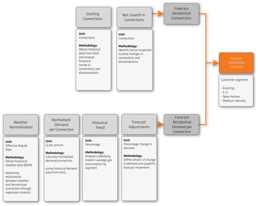
Demand and Customer Forecast Table of Contents

List of Figures
Figure 1.1. CORE Methodology – Tariff R and Tariff C. .................................................................................................. 13

Figure 1.2. CORE Methodology - Tariff D. ....................................................................................................................... 13

Figure 1.3. Total Volume Tariff Demand .......................................................................................................................... 14

Figure 1.4. Total Volume Tariff Connections ................................................................................................................... 14

Figure 1.5. Total Tariff D MDQ | GJ .................................................................................................................................. 15

Figure 1.6. Total Tariff D ACQ | GJ ................................................................................................................................... 15

Figure 1.7. Forecast Benchmarking | Residential Demand per Connection................................................................. 17

Figure 1.8. Forecast Benchmarking | Residential Connections .................................................................................... 17

Figure 2.1. Seasonal Demand Pattern | Manufacturing Sector Average Monthly ACQ ............................................... 22

Figure 2.2. Seasonal Demand Pattern | Education and Training Sector Average Monthly ACQ ................................ 22

Figure 2.3. Tariff R Residential Demand Forecast Methodology ................................................................................... 24

Figure 2.4. Tariff C Commercial Methodology ................................................................................................................ 27

Figure 2.5. Tariff D Industrial Methodology ..................................................................................................................... 30

Figure 3.1. EDD Index ........................................................................................................................................................ 33

Figure 3.2. Residential Demand per Connection | GJ..................................................................................................... 34

Figure 3.3. Residential Demand | GJ ................................................................................................................................ 34

Figure 3.4. Commercial Demand per Connection | GJ ................................................................................................... 34

Figure 3.5. Commercial Demand | GJ .............................................................................................................................. 34

Figure 3.6. Tariff D Weather Group- Demand per Connection | GJ ............................................................................... 36

Figure 4.1. SA Dwelling Completions by Dwelling Type ................................................................................................ 39

Figure 4.2. Greater Adelaide Population Growth | % ...................................................................................................... 39

Figure 4.3. New Residential Connections (LHS, No.) versus Penetration Rate of New Dwellings (RHS, %) ............. 39

Figure 6.1. Industrial MDQ | GJ ........................................................................................................................................ 51

Figure 6.2. Industrial Annual Demand | GJ ...................................................................................................................... 51

Figure 6.3. Industrial Customer Numbers | No................................................................................................................ 51

Figure 7.1. Industrial MDQ | GJ ........................................................................................................................................ 54

Figure 7.2. Industrial Annual Demand | GJ ...................................................................................................................... 54

Figure 7.3. Industrial Connections | GJ ........................................................................................................................... 54

Figure 7.4. Commercial Demand | GJ p.a. ....................................................................................................................... 55

Figure 7.5. Commercial Connections | No. ...................................................................................................................... 56

Figure 7.6. Commercial Existing Connections | No. ....................................................................................................... 56

Figure 7.7. Commercial Net Connections | No. ............................................................................................................... 57

Figure 7.8. Commercial New Connections | No. ............................................................................................................. 57

Figure 7.9. Commercial Total Demand per Connection | GJ/conn ................................................................................ 58

© CORE 2020 July 2020 v
Demand and Customer Forecast Table of Contents

Figure 7.10. Commercial New Demand per Connection | GJ/conn ................................................................................. 58

Figure 7.11. Residential Demand | GJ ................................................................................................................................ 59

Figure 7.12. Residential Total Connections | No. .............................................................................................................. 60

Figure 7.13. Residential Existing Connections | No. ........................................................................................................ 60

Figure 7.14. Residential New Connections | No. ............................................................................................................... 61

Figure 7.15. Residential Net Connections | No. ................................................................................................................ 61

Figure 7.16. New Residential Estate Connections | No. ................................................................................................... 61

Figure 7.17. New Residential E2G Connections | No. ....................................................................................................... 61

Figure 7.18. New Residential MDHR Connections | No. ................................................................................................... 61

Figure 7.19. Residential Demand per Connection | GJ/conn ........................................................................................... 62

Figure 7.20. Existing Demand per Connection | GJ/conn ................................................................................................ 62

Figure 7.21. New Residential Demand per Connection | GJ/conn ................................................................................... 63

© CORE 2020 July 2020 vi
Demand and Customer Forecast Glossary

Glossary
 AA Gas Access Arrangement Review

 ACT Australian Capital Territory

 AGIG Australian Gas Infrastructure Group

 AGN - SA Australian Gas Networks – South Australia

 AEMO Australian Energy Market Operator

 AER Australian Energy Regulator

 BOM Bureau of Meteorology

 CBJV Cooper Basin Joint Venture

 COAG Council of Australian Governments

 CORE Core Energy & Resources Pty. Limited

 DD Degree Days

 EDD Effective Degree Days

 EEO Energy Efficiency Opportunities

 E-to-G Electricity-to-Gas

 GBJV Gippsland Basin Joint Venture

 GEMS Greenhouse and Energy Minimum Standards

 HDD Heating Degree Days

 JCC Japanese Cleared Crude

 LGA Local Government Area

 LRET Large-scale Renewable Energy Target

 LRMC Long Run Marginal Cost

 MD Medium Density (Dwelling)

 MD/HR Medium Density/ High-Rise

 MDQ Maximum Daily Quantity

 MEPS Minimum Energy Performance Standards

 MAP Moomba to Adelaide Pipeline

 NABERS National Australian Built Environment Rating System

 NSW New South Wales

 RET Renewable Energy Target

 SA South Australia

 SRES Small Scale Renewable Energy Scheme

 STTM Short Term Trading Market

 VIC Victoria

 WA Western Australia

© CORE 2020 July 2020 7
Section 1 | Summary
Network Demand and Customer Forecast Section 1 1. Executive Summary

Section 1 | 1. Executive Summary

1.1. Scope of this Report
This report has been prepared by Core Energy & Resources Pty Ltd (“CORE”) for the purpose of providing Australian
Gas Networks (“AGN”) with an independent forecast of gas customers and demand for the company’s natural gas
distribution network in South Australia (“SA”), for the five financial years from 1 July 2021 to 30 June 2026 (“Review
Period”).

CORE has noted that these projections (both this Report and related forecasting models1) will form part of AGN’s Gas
Access Arrangement Review (“AA”) submission to the Australian Energy Regulator (“AER”).

CORE acknowledges that the derivation of mid to longer range forecasts generally, and this customer and demand
forecast specifically, involve a significant degree of uncertainty. Accordingly, CORE has taken all reasonable steps to
ensure this Report, and the approach to deriving the forecasts referred to within the Report, comply with Division 2 of
the National Gas Rules (“NGR”) "Access arrangement information relevant to price and revenue regulation", and in
particular, parts 74 and 75 as referenced below.

 "74. Forecasts and estimates

 (1) Information in the nature of a forecast or estimate must be supported by a statement of the basis of the
 forecast or estimate.

 (2) A forecast or estimate:

 (a) must be arrived at on a reasonable basis; and

 (b) must represent the best forecast or estimate possible in the circumstances.

 75. Inferred or derivative information

 Information in the nature of an extrapolation or inference must be supported by the primary information on which
 the extrapolation or inference is based." 2

1 The forecasting models are confidential, and an application will be sought for disclosure to be suppressed in accordance with NGR part 43 (2) (b).
2 NGR dated April 2014 and accessed from AEMC website.

© CORE 2020 July 2020 9
Network Demand and Customer Forecast Section 1 1. Executive Summary

1.2. Core Energy Group - Demand Forecast Experience
The following table outlines the experience held by members of CORE for both energy demand forecasting and
independent expert witness roles:

 Focus Area Experience

 ▪ A variety of independent expert roles covering:
 ˃ Gas contract disputes
 ˃ Gas price reviews – east and western Australia
 ˃ Gas demand – electricity, industrial, distribution, transmission
 Independent Expert/Witness ˃ Drilling activity (LNG)
 ˃ Gas processing plants
 ˃ Gas transmission pipelines
 ˃ Gas storage
 ˃ International LNG

 ▪ Development of models and analytical tools, forecasts and demand scenarios along the gas sector value
 chain:

 ˃ Exploration and production;
 ˃ Transmission;
 Demand forecasting, ˃ Distribution;
 modelling and scenario
 analysis ˃ Electricity generation;
 ˃ Retailing; and
 ˃ Liquefaction (LNG)

 ▪ Demand forecasting for a diverse range of clients including energy producers, gas infrastructure companies,
 retailers and the market operator (AEMO- in support of the GSOO publication).

 Access Arrangements
 ˃ WA – ATCO
 ˃ NSW – Jemena
 ˃ VIC – AGN
 Gas Distribution ˃ SA – Envestra (now AGN SA)
 ˃ ACT – ActewAGL (now Evoenergy)
 General
 ˃ Demand forecasting, modeling and scenario analysis covering all Australian networks

 ˃ Acquisition of Wagga Gas Network from NSW Government

 ▪ Development of gas demand scenarios for major transmission systems:

 ˃ South West Queensland
 ˃ Roma Brisbane
 ˃ Moomba Sydney
 Gas Transmission ˃ Eastern Gas Pipeline
 ˃ Moomba Adelaide
 ˃ SEAGas
 ˃ Tasmania
 ˃ QCLNG transmission line

 ▪ Development of contracted and potential demand and supply scenarios:
 ˃ Cooper Basin: SA and SWQ JV; unconventional gas (shale, coal seam, tight gas)
 ˃ Gippsland Basin: Gippsland Basin JV
 Gas Exploration and
 Production ˃ Otway Basin: Minerva, Thylacine-Geographe, Casino
 ˃ Surat/Bowen Basins: all major Queensland coal seam gas fields
 ˃ WA Basins: NWS Domgas, John Brookes, Gorgon, Wheatstone, Pluto
 ˃ LNG – NWS JV, Gorgon, Pluto, Ichthys, Wheatstone, GLNG, APLNG, QCLNG, Darwin LNG

© CORE 2020 July 2020 10
Network Demand and Customer Forecast Section 1 1. Executive Summary

1.3. Structure of Report
This report comprises two Sections:

Section 1 – Summary

A summary of the approach to forecasting network demand and customer numbers including:

 ▪ Methodology

 ▪ Tariff R and Tariff C Forecasts – connections/customer numbers and demand

 > Residential, Tariff R

 > Commercial, Tariff C

 ▪ Tariff D Forecast – Maximum Demand and ACQ Forecast

 ▪ Conclusion

Section 2 – Supporting Information and Analysis

Information and analysis undertaken by CORE to derive the forecasts set out in the Summary. This includes:

 ▪ Weather Normalisation

 ▪ Retail Gas & Electricity Price Forecast

 ▪ Price Elasticity of Demand

 ▪ Regression Analysis and Results

 ▪ Review of Appliance and Dwelling Efficiency; Associated Policy

 ▪ Review of Previous AA Forecast

Please note that all years referred to are financial years unless otherwise stated.

1.4. Overview of the AGN South Australia Network
The SA gas distribution network under review services around 455,000 customers with a mains length of
approximately 8,100 kilometres. The significant populations reached by the network include Adelaide, Whyalla, Port
Pirie, Nurioopta, Berri, Murray Bridge and Mount Gambier.3

For the purpose of this report, reference will be made to three customer segments - Tariff R, Tariff C and Tariff D as
defined in Table 1.1 below. The table also sets out the nature of the forecasts that CORE was asked to prepare.
These forecasts reflect the billing structure for each customer group. For example, forecasts of MDQ are not required
for residential customers as this group is charged based on the volume of gas used.

3 Source: Australian Gas Infrastructure Group 2018 Annual Review

© CORE 2020 July 2020 11
Network Demand and Customer Forecast Section 1 1. Executive Summary

1.4.1. Tariff Classification

For the purpose of this Report, reference will be made to three customer segments - Tariff R, Tariff C and Tariff D4 as
defined in Table 1.1 below.

Table 1.1. Customer Segments used for Tariff Classification.

 Customer Description
 segment

 Volume Tariffs – AGN’s Volume Tariff customer groups consist of Residential customers (Tariff R) and
 Tariff R, Tariff C Commercial customers (Tariff C) who are reasonably expected to consume less than 10 TJ
 (10TJ)
 Throughout this Report, the Demand Tariff customer group will be referred to as Tariff D
 customers and MDQ will be referred to for certain historical data and analysis- this refers to the
 highest day’s consumption within a particular year. ACQ refers to the total volume consumed
 within one year.
Source: CORE based on advice from AGN and AGN Schedule of Tariffs and Plans.

4 These types are consistent with the Volume Tariff and Demand Tariff customer groups used in tariff assignment as referenced in the 2020 AGN Schedule of
Tariffs and Plans.

© CORE 2020 July 2020 12
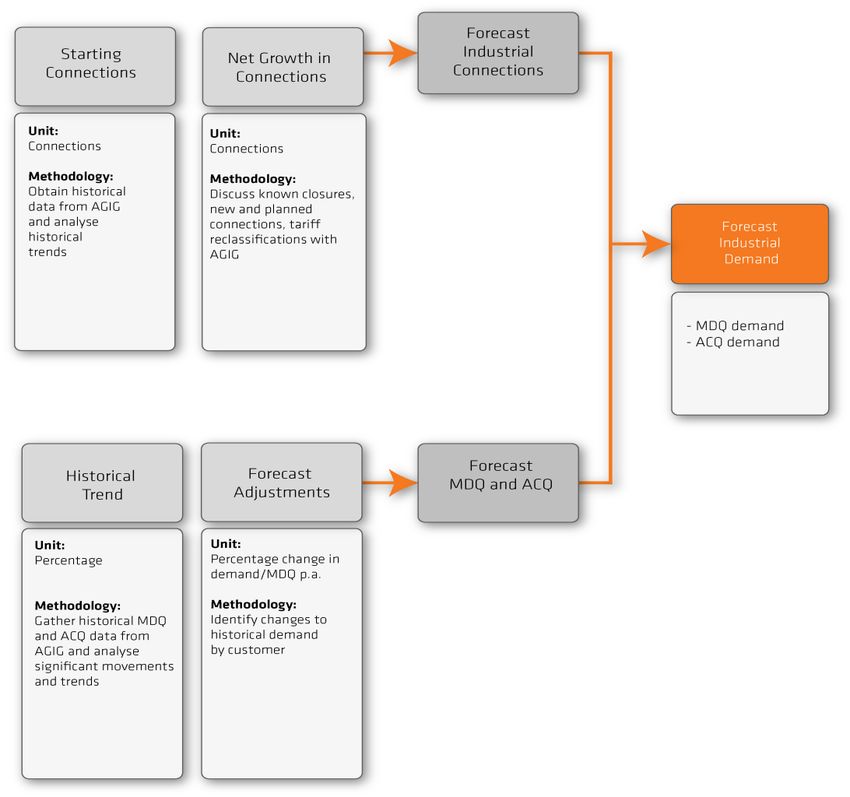
Network Demand and Customer Forecast Section 1 1. Executive Summary

1.5. Methodology Overview
An overview of the methodology adopted by CORE to derive forecasts of network demand and customer numbers is
provided below for both volume and demand customers. Further detail is presented in Section 2.

1.5.1. Volume Tariff Groups

Figure 1.1. CORE Methodology – Tariff R and Tariff C.

 Step 1
 Step 2 Step 3

 Identify material factors influencing Identify material factors influencing
 Normalise historic demand data to
 movement in demand per movement in net connections for
 remove influences of abnormal
 connection for each customer each customer segment and
 variations in weather and derive
 segment and collate data required collate data required to support
 extrapolation of normalised
 to support analysis and forecast of analysis and forecast of net
 Historic Trend
 demand per connection connections

 Step 4 Step 5
 Step 6
 Derive Adjusted Forecasts for
 Select preferred approach for connections and demand per Review and validate results
 quantifying all material factors connection for each customer through discussion with AGN and
 which are resonably expected to segment and provide explanation independent analysis, including
 drive forecast connections and of variance from normalised review of third party literature
 demand per connection Historical Trend (step 1)

Source: CORE.

1.5.2. Tariff D

Figure 1.2. CORE Methodology - Tariff D.

 Step 2
 Step 3
 Step 1
 Identify material factors influencing
 Select preferred approach for
 movement in individual demand
 forecasting material factors which
 per customer for the largest
 Compile list of individual customers are reasonably expected to drive
 customers (and by industry sector
 historical demand including MDQ, movements in demand including
 for remainder); collate data
 ACQ review of information from
 required to support analysis and
 network/customer engagement
 forecast of demand

 Step 5
 Step 4

 Review and validate results
 Derive forecast of demand through discussion with AGN and
 independent analysis, including
 review of third party literature

Source: CORE.

CORE is of the opinion that the rigorous application of this methodology, as presented within this Report, derives
forecasts which satisfy the requirements of the NGR - as the forecasts are derived on a reasonable basis, to provide
the best forecast or estimate possible under the circumstances, utilising appropriate primary information, where
available, to support the extrapolations/ forecasts.

© CORE 2020 July 2020 13
Network Demand and Customer Forecast Section 1 1. Executive Summary

1.6. Overview of History & Forecast for R and C Tariff Groups
Table 1.2 and Figure 1.3 provide a summary of actual connections, normalised demand per connection and total
normalised demand for both volume tariff groups, together with a summary of average annual growth.

Table 1.2. Historical Connections, Demand per Connection and Demand – Volume Tariff Groups.

 AAGR AAGR
 Closing Connections 2019 Historical 2026 Forecast
 09-19 H 22-26 F
 Residential 443,043 1.59% 476,549 1.04%
 Commercial 11,233 1.41% 11,644 0.62%
 Total Volume Tariff Connections 454,276 1.59% 488,192 1.03%
 Normalised Demand per Connection
 Residential 16.5 -2.03% 13.9 -2.55%
 Commercial 295.7 -0.44% 291.5 -0.30%
 Normalised Total Demand
 Residential 7,323,982 -0.45% 6,603,465 -1.54%
 Commercial 3,322,122 0.95% 3,394,132 0.31%
 Total Volume Tariff Demand 10,646,105 -0.06% 9,997,597 -0.93%

Source: CORE with historical data from AGN.

 Figure 1.3. Total Volume Tariff Demand Figure 1.4. Total Volume Tariff Connections
 12,000,000 600,000

 10,000,000 500,000

 8,000,000 400,000

 6,000,000 300,000

 4,000,000 200,000

 2,000,000 100,000

 - -
 2009 2013 2017 2021 2025 2009 2013 2017 2021 2025

 The contribution from Tariff R is shown via the grey dashed lines; The contribution from Tariff C is represented by the remaining proportion above the line.

 Source: CORE with historical data from AGN.

© CORE 2020 July 2020 14
Network Demand and Customer Forecast Section 1 1. Executive Summary

1.7. Overview of Historical Tariff D Demand
The following table and figures provide a summary of historical and forecast ACQ and MDQ demand for Tariff D,
together with a summary of average annual growth rates.

Table 1.3. Tariff D Demand Projection | Summary

 Tariff D AAGR AAGR
 2019 Historical 2026 Forecast
 Demand (GJ) 09-19 H 22-26 F

 ACQ 11,366,654.3 -2.09% 9,144,673.9 -2.85%

 MDQ 50,486 -2.39% 39,174 -3.12%

Source: CORE based on historical data from AGN.

 Figure 1.5. Total Tariff D MDQ | GJ Figure 1.6. Total Tariff D ACQ | GJ
 70,000 16,000,000

 60,000 14,000,000

 12,000,000
 50,000
 10,000,000
 40,000
 8,000,000
 30,000
 6,000,000
 20,000
 4,000,000

 10,000 2,000,000

 - -
 2010 2014 2018 2022 2026 2010 2014 2018 2022 2026

Source: CORE with historical data from AGN.

1.8. Overview of Connections and Demand Forecast
The following paragraphs provide a summary of the forecasts derived by CORE for all customer types.

1.8.1. Tariff R and Tariff C

Gas demand for volume customers is forecast to decrease at an annual average of -0.93% from 2022 to 2026. This
forecast is influenced by two principal forces - an increase in connections of 1.03% p.a., offset by a reduction in
demand per connection of -1.94% p.a. The contribution from each customer group is shown in the following table:

© CORE 2020 July 2020 15
Network Demand and Customer Forecast Section 1 1. Executive Summary

Table 1.4. Volume Tariff Connections, Demand per Connection and Demand | Summary
 AAGR AAGR
 2022 2022 2023 2024 2026
 2009-2019 2022-2026
 Connections

 Residential 455,278 459,953 465,169 470,924 476,549 1.59% 1.04%

 Commercial 11,231 11,337 11,442 11,544 11,644 1.41% 0.62%

 Total 466,509 471,290 476,611 482,468 488,192 1.59% 1.03%

 Demand Per Connection

 Residential 15.5 15.1 14.7 14.3 13.9 -2.03% -2.55%

 Commercial 299.3 298.9 297.0 293.9 291.5 -0.44% -0.30%

 Total 22.3 21.9 21.5 20.9 20.5 -1.62% -1.94%

 Total Demand

 Residential 7,060,676 6,955,659 6,837,687 6,713,646 6,603,465 -0.46% -1.54%

 Commercial 3,361,039 3,388,745 3,398,272 3,392,675 3,394,132 0.95% 0.31%

 Total 10,421,715 10,344,404 10,235,959 10,106,321 9,997,597 -0.06% -0.93%

Source: CORE Demand Forecast

The major factor contributing to the reduction in volume customer demand is a reduction in demand per connection for
residential customers, which is influenced by:

 ▪ continued growth in share of connections for medium and high-density connections which exhibit lower gas usage
 per dwelling;

 ▪ continued trends in gas appliance and dwelling efficiency, contributing to reductions in demand per connection;

 ▪ customer demand response to gas and electricity price movements whereby electricity prices are projected to
 move more favourably than gas during the forecast period; and

 ▪ reduced space heating usage attributable to competition with alternative energy sources, including R-C air-
 conditioning.

1.8.2. Tariff D

Capacity demand (as measured by MDQ) for Tariff D customers is forecast to fall by an annual average of -3.12%
p.a. from 2022 to 2026 as shown in the table below. This fall is attributable to a continued reduction in gas-intensive
industrial capacity and an increase in operational energy efficiencies at the individual plant level. Due to billing cycle
lag and variability as to economic impact and recovery, CORE was unable to quantifiably modify the forecast to
capture the impact of COVID. However, the impact of the COVID pandemic represents significant downside risk,
particularly to large space heating customers (closed shopping centres and leisure centres) and manufacturers at risk
of negative demand shocks.

Table 1.5. Tariff D Demand Projection | Summary
 AAGR AAGR
 Tariff D 2022 2023 2024 2025 2026
 2009-2019 2022-2026

 MDQ 44,422 43,008 41,659 40,380 39,174 -2.39% -3.12%

 ACQ 10,269,515 9,979,838 9,695,806 9,417,434 9,144,674 -2.09% -2.85%

Source: CORE, utilising historical data from AGN.

© CORE 2020 July 2020 16
Network Demand and Customer Forecast Section 1 1. Executive Summary

The decline in MDQ is modelled to continue its decline albeit at a slower long-term rate than the historical period
although short term COVID pandemic demand shocks within the South Australian economy could result in larger
declines:

 ▪ known and projected business closures/ capacity reductions are expected to be smaller relative to the reductions
 that occurred during the historical period; and

 ▪ continuing trend in energy efficiency, including peak demand as a response to increased energy costs and profit
 pressures more broadly.

1.9. Validation
An important part of the work program undertaken by CORE in relation to the derivation of AGN forecasts is a
validation process. This involves CORE identifying independent third-party analysis which addresses one or more
factors considered by CORE in deriving a final forecast. This validation process has been applied in a range of areas
including, but not limited to:

 ▪ estimates of residential dwelling trends in South Australia including dwelling type and overall growth;

 ▪ projections of retail gas and electricity prices for South Australian customers;

 ▪ trends in energy efficiency at the appliance and building level; and

 ▪ trends in the South Australian economy such as economic output, business formation and manufacturing activity.5

In addition, CORE has reviewed all recent demand forecasts which have formed part of final AA decisions for other
networks in Eastern Australia, to determine whether trend forecasts are consistent with other networks. The following
charts show that the residential forecast (the majority of volume and connections) is forecast to move in the same
direction as all other eastern networks with annual growth rates that are typical of other networks. It should be noted
that the slowest decline in demand for connection shown for JGN is due partly to growth in a new multi-dwelling meter
type whereby one metered connection is typically supporting 50-100 individual dwellings. The following sections will
discuss the drivers of this forecast and demonstrate a consistency with own-history and neighbouring jurisdictions.

 Figure 1.7. Forecast Benchmarking | Residential Demand Figure 1.8. Forecast Benchmarking | Residential Connections
 per Connection

 0.00% 4.00%
 AGN South Australia AGN South Australia
 -0.50% 3.50%
 Evoenergy ACT Evoenergy ACT
 -1.00% 3.00%
 AGN Victoria & AGN Victoria &
 -1.50% 2.50%
 Albury Albury

 -2.00% Ausnet Victoria 2.00% Ausnet Victoria

 -2.50% Multinet Victoria 1.50% Multinet Victoria

 -3.00% 1.00%
 APT Allgas APT Allgas
 Queensland Queensland
 -3.50% 0.50%
 JGN JGN
 -4.00% 0.00%

5
 These macroeconomic drivers are exposed to significant downside risk due to the ultimate impact of the COVID pandemic, an impact that was not yet visible
when analysis was undertaken.

© CORE 2020 July 2020 17
Demand and Customer Forecast Section 1 2.Methodology

Section 1 | 2. Methodology
The methodology adopted by CORE to derive a gas demand forecast for the South Australian gas distribution
network, involves four primary elements. Each element is expanded upon in the relevant section of this report.

 1 An approach to normalising historical demand to remove the impact of abnormal weather and prices

 2 An approach to deriving a forecast of Residential demand

 3 An approach to deriving a forecast of Commercial demand

 4 An approach to deriving a forecast of Tariff D Industrial demand

The methodology adopted by CORE considers all recent AA demand forecast proposals, draft decisions and final
decisions, which allowed the development of a best-practice approach whilst also remaining compliant with the NGR.

The methodology favours a highly transparent approach, including a demand forecast model that examines all factors
that could potentially impact normalised demand. This approach is fundamentally consistent with the methodology
presented by AEMO in its latest National Gas Forecasting Report (“NGFR”).6

This report sets out the underlying facts and assumptions that were necessary when analysing gas demand. The
requested comprehensive data set as provided by AGN covers the 2009 to 2019 period, enabling CORE to review at
least one full decade of historical trends for the volume tariff class and demand tariff class. CORE was also able to
append the pre-2009 mass market historical trends observed and approved for the prior GAAR submission. This has
enhanced the forecast by incorporating a longer time period of demand drivers and reduces the impact of one-off
fluctuations. Tariff D analysis is performed on an individual customer basis with more focus on recent/proposed
operational changes and macroeconomic influences hence a 10-year history was deemed a sufficient period for this
forecast.

CORE considers this process to be compliant with s 74(2) of the NGR. Forecasts are constructed on a reasonable
basis whilst representing the best forecasts possible in the circumstances.

Tariff R Residential and Tariff C Commercial demand is derived by multiplying the forecast number of connections by
the forecast demand per connection, for each customer segment. This results in separate forecasts for each customer
type (residential versus) and connection type (new versus existing connections; further broken down into different
types of new dwelling). Tariff D Industrial demand was completed on an individual customer basis with customers
sorted according to size, ANZSIC division and demand pattern (e.g. macroeconomic influence and/or weather-
induced demand). Further details of approach are set out below for residential, commercial and industrial tariff
classes.

6
 NGFR now delivered as part of the GSOO publication. Refer to Gas Demand Forecasting Methodology Information Paper, March 2019

© CORE 2020 July 2020 18
Demand and Customer Forecast Section 1 2.Methodology

2.1. Weather Normalised Demand
Gas demand is materially influenced by weather, particularly in the residential sector. Accordingly, the weather impact
on historical residential and commercial demand was normalised to provide an appropriate basis for demand
forecasting. CORE adopted a weather normalisation methodology based on AEMO’s forecasting guidelines7, which
favours the application of Effective Degree Days (“EDD”). In comparing the methods of Heating Degree Days ("HDD")
and EDD, EDD accounts for additional climatic factors such as:

 ▪ Sunshine hours.

 ▪ Wind chill; and

 ▪ Seasonality.

The coefficient of determination calculated by CORE also showed that EDD has a stronger relationship with gas
demand than HDD. In addition, the Akaike Information Criterion (“AIC”) supports the use of EDD instead of HDD as
an index of weather fluctuations. For these reasons, CORE used EDD as a superior approach to weather
normalisation.

2.1.1. EDD Index

The weather index selected for weather normalisation was based on AEMO’s EDD312 methodology which has been
approved by the AER in a number of previous gas access arrangements (“AA”). AEMO has endorsed the EDD312 as a
more rigorous approach than EDD129 or HDD indices. The calculation method and resulting parameters are outlined
below:

EDD Calculation:

1. Develop an EDD Index Model that calculates the EDD Index coefficients – this model is included as a supporting
 document to this report.

2. Derive EDD Index coefficients by regressing daily gas demand on climate data, ranging from 2005 to 2019. The start
 date of the regression was based on the availability of reliable daily gas demand data which spanned 15 years -
 deemed appropriate by CORE. Historical climate data for the Adelaide metropolitan area was obtained from the Bureau
 of Meteorology (temperature, wind speed, sunshine hours) who recorded the available data points at major Adelaide
 weather stations during the historical series (West Terrace, Kent Town and Adelaide Airport). CORE has analysed the
 historical relationship of sunshine hours between the three stations and come up with an adjustment factor such that
 one consistent historical series was derivable. Most climate observations used came from the Kent Town Weather
 Station and missing data was substituted using West Terrace or Adelaide Airport readings (corrected by an adjustment
 factor).8 The average daily temperature and wind speed data was estimated using the average of 8x3-hourly data
 between 3.00 am and 12.00 am Dummy variables for certain days of the week (Friday, Saturday and Sunday) were also
 included in the regression to capture the additional gas demand that occurs on Sundays and the reduced demand that
 occurs on Fridays and Saturdays.9

7
 AEMO, 2012 Weather Standards for Gas Forecasting.
8
 Weather Station 023090. CORE notes that the distribution network includes customers located some distance from Adelaide. However, the majority of
customers are located in the Greater Adelaide area hence the weather observations for Adelaide Metro are appropriate, as has been approved by the AER
previously. CORE notes that the AER has accepted this approach in Vic and NSW for networks that also have significant latitude ranges and customers located
at different altitudes.
9
 Main difference in activity includes business opening hours and the number of hours residents spend at home cooking and using space heaters.

© CORE 2020 July 2020 19
Demand and Customer Forecast Section 1 2.Methodology 3. Calculate EDD by using the weather normalised demand model and derived EDD index coefficients. The weather normalisation model is included as a supporting document to this report. Below are the model structure and coefficients of CORE’s EDD312 Index: Daily demand per connection = b0 + b1*EDD + b2*Friday + b3*Saturday +b4*Sunday. EDD = Degree Day (“DD312”) temperature effect + 0.0242 * DD312*average wind speed wind chill factor - 0.10 * sunshine hours warming effect of sunshine 2π(day−201) seasonality factor + max(3.58*2* Cos ( )) 365 Where DD312 is the degree day as calculated by the following table: DD312 = T2 – T1 if T1 < T2 Daily temperature above threshold temperature 0 if T1 > T2 Daily temperature below threshold temperature ▪ T1 is the average of 8 three-hourly temperature readings (in degrees Celsius) from 3.00am to 12.00am from the Bureau of Meteorology’s Kent Town Weather Station- deemed by CORE to be an appropriate weather station for the network. ▪ T2 is equal to 18.49 degrees Celsius and represents the estimated threshold temperature for gas heating within the AGN SA Network. ▪ Average wind speed is the average of the 8 three-hourly wind observations (measured in knots) from 3.00am to 12.00am measured at the Kent Town Weather Station. ▪ Sunshine hours are the number of hours of sunshine above a standard intensity as measured at the Weather Bureau’s Kent Town Weather Station until June 2015 when this dataset was discontinued. To complete the historical series, observations from Adelaide Airport were used with a correction factor (derived from historical periods where both weather stations recorded this data point).10 ▪ The seasonality factor models variability in consumer response to different weather. It indicates that Residential and Commercial consumers more readily turn on, adjust heaters higher or leave heaters on longer in winter than in the shoulder seasons given the same weather or change in weather conditions. For example, central heaters are often programmed once cold weather sets in resulting in more regular use and consumers are potentially in the habit of using heating appliances once the middle of winter is reached. This change in consumer behaviour is captured in the Cosine term in the EDD formula, which implies that for the same weather conditions heating demand is higher in winter than in the shoulder seasons or in summer.11 10 CORE has set this coefficient to 0.10 as this provided a higher R squared result than a coefficient of 0 which was the coefficient achieved using the Excel Solver add-in. Given the higher predictive power and greater consistency with historical precedent (e.g. prior AA), the decision was made to use 0.10 rather than defer to the 0 coefficient which was likely being achieved due to an upper limit of iterations imposed by Solver. The same process was applied to other variables, but this did not lead to a superior statistical result. 11 As described in; AEMO, Victorian EDD Weather Standards – EDD312 (2012) © CORE 2020 July 2020 20
Demand and Customer Forecast Section 1 2.Methodology

2.1.2. Weather Normalised Demand Model

The EDD312 Weather Index was then used for regression analysis on AGN residential and commercial demand data.

 Residential and commercial data was regressed separately on historical EDD data, on a
 1.
 monthly basis

 The optimum statistical relationship between customer gas demand and weather
 2. fluctuations was obtained

 The regressions were performed with the two main data sets:
 3. ▪ Monthly sum of EDDs (calculated from the daily EDD series obtained from the first stage)
 ▪ Monthly sum of gas demand (AGN demand data)

A variety of model specifications and model terms were tested for their predictive power and statistical rigour,
including:

 ▪ Lagged values of the gas demand data

 ▪ Logarithmic and differencing transformations of the weather/demand data

 ▪ Variables that capture the impact from events specific to one part of the data series (dummy variables)

Please see Appendix A1 for a full summary of the regression model output and statistical test results. The statistical
models selected for the forecast of residential and commercial demand satisfied the following criteria:

 Explanatory Variables
 significant at 5% confidence
 level

 Explanatory Variables have Model passes key
 intuitive sign based on econometric tests,
 established theory acceptable rigour

 Model has suitable Model variables can reasonably
 AIC relative to be expected to have a significant
 candidate models impact on gas demand

 Statistical Model Selection

© CORE 2020 July 2020 21
Demand and Customer Forecast Section 1 2.Methodology

CORE considers this process to be compliant with s 74(2) of the NGR. Forecasts are constructed on a reasonable
basis whilst representing the best forecasts possible in the circumstances.

2.2. Weather Normalisation | Tariff D
In addition to the residential and commercial tariff groups detailed in the previous section, CORE adopted the same
methodology to weather normalise a portion of the industrial tariff group. After segregating these customer groups into
their respective ANZSIC code sectors, it was clear that certain sectors exhibit strong weather-induced patterns
whereas others do not. For instance, the following charts compare the monthly sum of demand for manufacturing
customers and industrial customers within the Health Care & Social Assistance sector. For manufacturers there are
fluctuations around December and January which are typically driven by maintenance periods and reduced operations
during the festive season. In comparison, the Health & Social Assistance sector comprises large medical facilities and
residential premises which exhibit a strong winter peak. For this sector, weather-induced heating load is a key
determinant.

 Figure 2.1. Seasonal Demand Pattern | Manufacturing Sector Figure 2.2. Seasonal Demand Pattern | Education and Training
 Average Monthly ACQ Sector Average Monthly ACQ

 350,000 6,000

 300,000
 5,000

 250,000
 4,000

 200,000
 3,000
 150,000

 2,000
 100,000

 1,000
 50,000

 - -
 Jan Feb Mar Apr May Jun Jul Aug Sep Oct Nov Dec Jan Feb Mar Apr May Jun Jul Aug Sep Oct Nov Dec

CORE then weather normalised the following industrial customer groups:

 ▪ Accommodation and Food Services

 ▪ Professional, Scientific and Technical Services

 ▪ Administrative and Support Services

 ▪ Public Administration and Safety

 ▪ Education and Training

 ▪ Health Care and Social Assistance

 ▪ Arts and Recreation Services

 ▪ Other Services

© CORE 2020 July 2020 22
Demand and Customer Forecast Section 1 2.Methodology

The remaining sectors were forecast using GVA12, GSP13 and other regression analysis (refer Appendix A4 for
additional details):

 ▪ Agriculture, Forestry & Fishing

 ▪ Mining

 ▪ Manufacturing

 ▪ Electricity, Gas, Water and Waste Services

 ▪ Construction

 ▪ Wholesale Trade

 ▪ Retail Trade

 ▪ Transport, Postal and Warehousing

 ▪ Information Media and Telecommunications

 ▪ Financial and Insurance Services

 ▪ Rental, Hiring and Real Estate Services

Statistical model types, regression post-estimation and overall methodology was consistent with the previous
description for Tariffs R and C above. Please refer to Appendix A1 and A4 for a full description of weather
normalisation regression analysis and results.

CORE notes that the approach is consistent with AEMO’s GSOO 2019 methodology whereby GVA is used to project
annual volume and large customers are individually analysed, separate to the trends applied to the pool of smaller
industrials. CORE notes also that the same econometric model (natural logarithmic transformation) was used by
AEMO to derive the relationship between ACQ and sector output.14

12
 Gross Value Add refers to the economic output of an economic sector
13
 Gross State Product refers to the economic output of a State/Territory
14
 Gas Demand Forecasting Methodology Information Paper, March 2019

© CORE 2020 July 2020 23
Demand and Customer Forecast Section 1 2.Methodology

2.3. Volume Tariffs Demand Methodology

2.3.1. Residential | Tariff R

The figure below provides a diagrammatic representation of the approach used by CORE to derive a forecast of Tariff
R demand, including a forecast of connections and demand per connection.

Figure 2.3. Tariff R Residential Demand Forecast Methodology

Source: CORE.

2.3.1.2. Connections

This section details the approach undertaken to derive residential connections. Due to the different types of dwellings,
CORE reconciles bottom-up and top-down approaches based on the connection type (e.g. single estate, medium-
density, high-rise). Separate analysis is also undertaken for the pool of existing connections versus a forecast of new
connections. The integration of third-party forecasts is inherent to this approach and provides a natural source of
validation.

 ▪ The bottom-up approach analyses historical trends and major factors which influence gas connections; and

© CORE 2020 July 2020 24
Demand and Customer Forecast Section 1 2.Methodology

 ▪ The top-down approach surveys the relevant forecasts completed by qualified third parties. The specific focus here is on
 dwelling completions within the distribution network.

Generally, each dwelling type exhibits its own growth cycle. By including a bottom-up approach, the total connections
forecast will likely be more accurate. This is consistent with other views within the industry such as AEMO who noted
that underlying causes of growth cannot be ascertained when distribution businesses report aggregated customer
numbers - the full picture of growth only becomes apparent when each dwelling type is separated. 15 CORE agrees
with AEMO’s views in regard to the distinct growth factors for different dwelling types. The method specific to each
dwelling type is outlined as follows:

Existing Connections

 ▪ Residential connection numbers were compiled by CORE based on data provided by AGN- including disconnections,
 net and gross/new connections.

 ▪ The closing 2019 connections are defined as existing connections in the forecast. This forms a basis to derive a forecast
 for the period 2020 to 2026. The forecast of existing connections for a given year is derived by removing the predicted
 disconnections in the previous year from the opening number of connections in the previous year. Forecast
 disconnections are based on the historical average of disconnections as a percentage of the year-opening number of
 connections.

 ▪ There are meters on the AGN SA Network for which there is no associated demand. This situation may occur if a
 property is vacant or if supply has been cut off as a result of non-payment. A significant removal program has been
 disclosed to CORE that will remove zero-consuming meters (“ZCMs”) at the outset of the forthcoming review period if
 the meter has continued in a state of non-consumption for the previous two years. An adjustment has been made to the
 forecast to capture this impact.

New Connections

CORE has derived an estimate of new dwelling connections in the 2022 to 2026 period via a four-step process:

1. Estimate new dwellings in SA

 > CORE has undertaken an extensive literature search as a basis for projected dwelling completions. Additionally,
 CORE has incorporated an independent third-party housing starts forecast published by HIA. This historical and
 forecast series indicates that the 2018 increase in new dwellings growth in SA was underpinned by MDHR
 activity. It had been expected that new dwellings will remain at or slightly above 2015-2017 levels after
 significant increases in 2018 followed by a correction in 2019. However, the impacts of the COVID pandemic
 give rise to a projection that 2021 dwelling commencements will decrease significantly. Given the uncertainty
 associated with economic recovery, CORE has opted to install a gradual recovery between 2022 and 2024.

 > The key results of this forecast are that total new dwellings growth is expected to remain steady for 2020
 (sufficient activity prior to pandemic commencement in March 2020), fall steeply in 2021 and return to 2015-2017
 levels by 2024.

2. Estimate the proportion of new SA dwellings within AGN’s area that will be connected to the gas network

 > CORE has undertaken analysis of the historical AGN SA Network penetration rate and applied this to the
 forecast of SA new dwellings.

15
 AEMO, Forecasting Methodology Information Paper, December 2014.

© CORE 2020 July 2020 25
Demand and Customer Forecast Section 1 2.Methodology

3. Determine the apportionment of network connected dwellings in the AGN area that are single versus medium density/
 high-rise dwellings

 > CORE has undertaken analysis of the historical average increase of each connection type and then applied HIA
 dwelling type projections to arrive at a new dwelling forecast by connection type. MD/HR is a faster growing
 source of new dwellings and AGN captures a lower percentage of these dwellings relative to single estates.

2.3.1.3. Demand per Connection

CORE has undertaken a qualitative assessment of the alternative methodologies which can reasonably be used to
derive a forecast of Demand per Connection for the Residential segment of the AGN SA Network. CORE has
determined that an approach which analyses the Historical Trend and adjusts for the impact of each material factor
which is reasonably expected to influence Demand per Connection (with appropriate rigour and data quality), to be
the best available approach under the AA circumstances. Further, CORE is of the opinion that such analysis must be
set out in a transparent fashion using a model which clearly sets out assumptions/ inputs, calculations and results, in
a manner which facilitates efficient scenario and sensitivity analysis.

Therefore, the steps taken to arrive at forecast demand per connection are as follows:

1. Develop models for calculation of EDD, normalised demand and forecast of Demand per Connection (these have been
 provided to AGN).

2. Normalise total demand per annum for the effects of weather using the methodology discussed in Section 1| 3.

3. Divide total historical demand by number of connections to determine average demand per connection. This includes an
 assessment of the relative demand per connection exhibited by different connection types (new versus existing; new
 detached estate versus E2G, medium-density/ high-rise).

4. Determine the historical trends in demand per connection, by connection type.

5. Derive an adjusted forecast of demand per connection having regard to the historical trend and the influence of factors
 which are not present in the historical trend.

Section 1.3 presents a detailed description of this process.

2.3.1.4. Forecast Demand

The product of forecast residential connections and forecast demand per residential connection is total forecast
demand for the Tariff R residential segment. CORE notes that its approach is consistent with the volume market
forecasting methodology relied upon by the market operator AEMO. AEMO also use dwelling completion forecasts to
project new connections and has also reverted to a historical average connections trend for non-residential
connections (just as CORE did after reviewing the historical volatility in the gross new connections series and
relationship with historical GSP). AEMO’s trend in demand per connection is primarily driven by a weather normalised
trend (same EDD312 methodology as CORE) and price responses. However, CORE notes that an ex-post adjustment
was then made to account for energy/appliance trends and climate change. CORE has reviewed available data sets
and believes historical trends captured in the weather normalised demand per connection series, sufficiently
incorporate the anticipated and continuing impact of these drivers in the AA period (noting that AEMO has to account

© CORE 2020 July 2020 26
You can also read