Investors and Housing Affordability y - Carlos Garrigaz, Pedro Getex, Athena Tsouderou February 2021 - IE
←
→
Page content transcription
If your browser does not render page correctly, please read the page content below
Investors and Housing A¤ordability y

                      Carlos Garrigaz, Pedro Getex, Athena Tsouderou{

                                             February 2021

                                                  Abstract

          This paper studies the impact of a new and growing class of institutional investors on
      U.S. housing a¤ordability. We …nd that investors’purchases increase the price-to-income
      ratio, especially in the bottom price-tier, the entry point for …rst-time buyers. Investors
      cause a short-run reduction in the vacancy rate and a medium-run positive response of
      construction, which is stronger for multi-unit buildings. The supply response mitigates
      the e¤ect on a¤ordability, although not enough to reverse the e¤ect. The transmission
      channels depend on the housing supply elasticity. In highly elastic areas investors a¤ect
      rents more than prices, whereas in highly inelastic areas investors have the opposite e¤ect.

          Keywords: Institutional investors, housing a¤ordability, house prices, supply elasticity,
      propensity to invest.

      We thank Itzhak Ben-David, Morris Davis, Anthony DeFusco, David Echeverry, Andra Ghent, Jonathan
Halket, Lu Han, Nina Karnaukh, Finn Kydland, Jose Maria Liberti, David Ling, Christos Andreas Makridis,
Charles Nathanson, Michael Reher, Stephen L. Ross, Martin Schneider, and participants at Durham, ECB,
Hebrew University of Jerusalem, NEOMA, Notre Dame, IE, Ohio State, and 2018 UEA, 2019 HULM, 2019
AREUEA International, 2019 AEFIN Finance Forum, 2019 SED, 2020 Econometric Society and 2020 AREUEA
Conferences.
    y
      The views expressed herein do not necessarily re‡ect those of the Federal Reserve Bank of St. Louis or the
Federal Reserve System. The results and opinions are those of the authors and do not re‡ect the position of
Zillow Group. Research reported in this paper was partially funded by the Spanish Ministry of Economy and
Competitiveness (MCIU), State Research Agency (AEI) and European Regional Development Fund (ERDF)
Grant No. PGC2018-101745-A-I00.
    z
      Federal Reserve Bank of St. Louis. carlos.garriga@stls.frb.org.
    x
      IE Business School, IE University. pedro.gete@ie.edu.
   {
      IE Business School, IE University. athenatsouderou@gmail.com.

                                                       1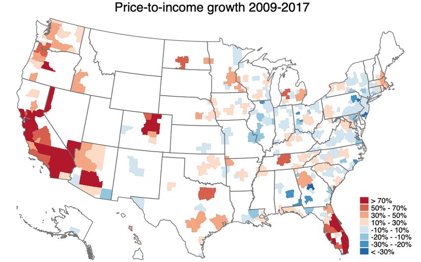
1 Introduction
Housing a¤ordability is one of the most pressing challenges for most cities in the world. In
the United States in 2019, the median house price exceeded three times the median household’s
annual income in 55% of the MSAs. Moreover, in 42% of the MSAs in 2019 the rent-to-income
ratio exceeded the threshold of rental a¤ordability of 27%. As Figure 1 shows, the recent lack
of housing a¤ordability resembles the situation during the large housing boom of the 2000s.
This paper studies the link between the recent worsening of a¤ordability and the emergence
of a new class of investors in real estate markets, namely, institutional investors. Increasing
demand from investors can move house prices directly, but it can also impact the rental market
by a¤ecting the supply of tenant-occupied housing. Investors’purchases can also in‡uence the
characteristics of the newly constructed units, for example favoring small or multi-family units
instead of more traditional single-family. Investors can shape the composition of the stock of
residential housing and can alter homeownership rates (Halket, Nesheim, and Oswald 2020).
There is a growing literature studying housing investors, like Agarwal et al. (2019), Cvi-
janovic and Spaenjers (2020), DeFusco et al. (2018), Favilukis and Van Nieuwerburgh (2021)
and others that we discuss below. Our contribution is to show that post-…nancial crisis insti-
tutional investors a¤ected housing prices and a¤ordability. The impact of investors’purchases
di¤ers across market segments based on price-tiers, building sizes, and locations with di¤erent
supply restrictions. We connect the asset pricing perspective with the traditional view of af-
fordability from urban economics that focuses on geographical supply constraints (Glaeser and
Gyourko 2018; Molloy, Nathanson, and Paciorek 2020).
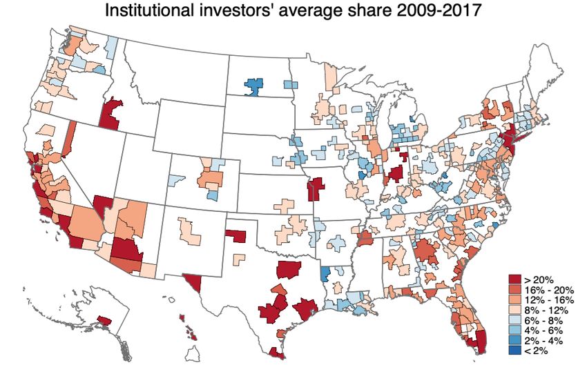
We de…ne institutional investors as legal entities who purchase multiple housing units under
the name of an LLC, LP, Trust, REIT, etc. Figure 2 shows a new fact: MSAs that experienced
the largest increase in the price-to-income ratio post-crisis also had the largest market share
of housing purchases by institutional investors.1 Establishing a causal connection is not direct.
For example a standard OLS regression of house price growth on investors’market share would
be biased downwards if investors were attracted to areas where prices collapsed following the
crisis. To overcome this challenge we use an instrumental variable approach with a rich dataset
covering the U.S. MSAs from 2000 to 2017.
We use a “Bartik inspired instrument”that takes advantage of the Quantitative Easing (QE)
programs that the Fed implemented during the …nancial crisis. QE resulted in a sharp decline
1
Figure A1 shows the positive correlation of the raw data in a scatter plot, also denoting the population of
each MSA.
2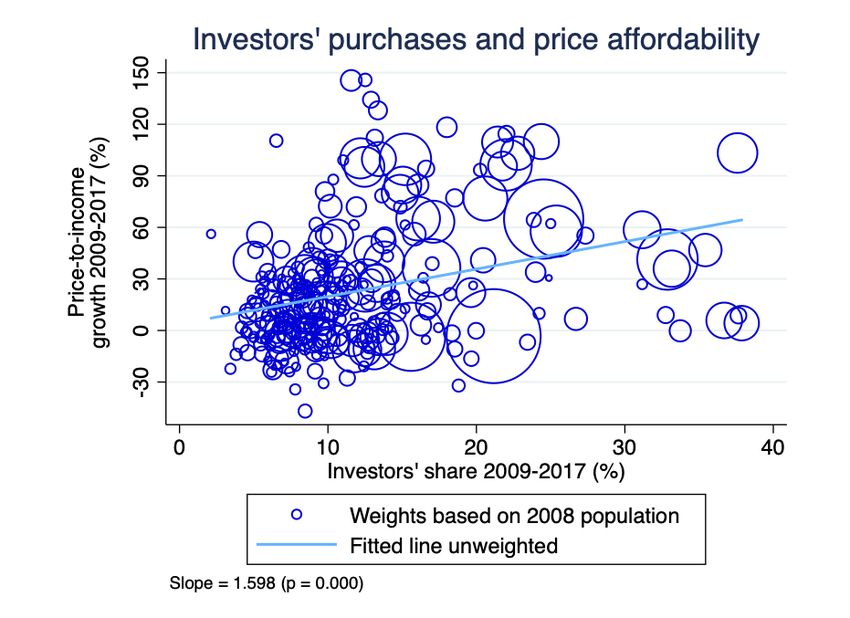
in the returns of safe assets, which encouraged risk-taking behavior by investors. Martínez-
Miera and Repullo (2017) and Rodnyansky and Darmouni (2017) document that QE triggered
a search for yield. While QE was a national shock, di¤erent regions reacted di¤erently based
on the pre-shock propensity for investments among the local high-income population. High-
earning, sophisticated residents directed more capital to the housing market, through new or
existing legal entities.

    We capture such pre-shock local propensity to invest with the share of the top earners’busi-
ness income over total income in each MSA in 2007. In the panel data analysis our instrument
is this share interacted with the growth rate in the rate on certi…cate of deposits (CDs). This
is like the housing net worth channel of Mian and Su… (2014) that exposes certain areas to
larger macro e¤ects from declines in housing prices due to their housing leverage. In our case,
we expose investment-prone areas to the QE national shock.

    It is straightforward to show that our instrument is strongly correlated with the geographical
presence of institutional housing investors post-crisis. The new housing investors post-crisis are
mainly small and local, and create legal entities to buy houses throughout the U.S., while the
large private equity investors’housing purchases are geographically concentrated in “superstar
cities” (Garriga, Gete, and Tsouderou 2020). Thus, the instrument satis…es the relevance
condition.

    We perform several tests to rigorously assess the exclusion restriction. That is, conditional
on observables, the share of the top earners’business income is uncorrelated with factors that
determine house prices: (1) We provide extensive evidence that in the pre-QE period the
instrument does not predict changes in housing prices or new construction. Areas with the
highest or lowest levels of the instrument exhibit parallel pre-trends. Placebo tests con…rm
that the instrument only captures post-crisis shocks to investment in the housing markets. The
assumption that there were no pre-existing di¤erences in the growth of housing prices and
that the common unconventional monetary policy shock caused the changes in price growth
seems plausible (Goldsmith-Pinkham, Sorkin, and Swift 2020). (2) We provide evidence that
it is very hard to predict the investment attitude of an MSA, as analogously it is di¢ cult to
explain which cities become hubs for entrepreneurship.2 That is, even if factors such as the tax
regime, natural amenities, or the structure of the population have some forecasting power, most
of the cross-sectional geographical variation in entrepreneurship, and in the share of business
income, is unexplained. Moreover, since the instrument is determined two years prior to the
period of study (2009 to 2017) this reduces risk of reverse causality. (3) We run a number
   2
   For example when trying to predict cross-regional di¤erences in entrepreneurship the largest R-squared in
Davidsson (1991) is 25%, and in Rocha and Sternberg (2005) is 23%.

                                                     3
of speci…cations to show that the results are not driven by shifts in the composition of labor
demand of MSAs during the post-crisis period. (4) We control thoroughly for an array of …xed
e¤ects and of local activity trends (income, population ‡ows, unemployment, GDP, wages and
labor force participation), so it is unlikely that the error term re‡ects common movers of both
investors and housing market variables. (5) Finally, we con…rm the robustness of the results to
alternative measures of the investors’presence and di¤erent geographical units.
Our …rst result is that institutional investors increase housing prices and worsen a¤ordability.
Between 2009 to 2017, one standard deviation higher purchases by institutional investors leads
to 1.46 percentage points higher housing price growth for the median house. Moreover, we …nd
that prices grow signi…cantly faster than income. Further investigation indicates that these
results do not come from the variation driven by the so-called “superstar cities” as discussed
by Gyourko, Mayer, and Sinai (2013), or by the purchases of so-called “Wall Street Landlords”
often discussed in the popular press.3 The analysis that excludes the top cities by large investors,
often correlated with superstar cities, still arrives to the same conclusions.
Housing markets are often segmented, hence, the e¤ect of house purchases might not have
the same pass-through across market tiers, consistent with evidence from Armesto and Garriga
(2009), and Piazzesi, Schneider, and Stroebel (2020). We …nd that the market segment that is
more sensitive to purchases by institutional investors is the bottom price-tier. In the bottom
price segment, one standard deviation higher purchases causes 2.29 percentage points higher
housing price growth. As …rst-time buyers tend to purchase housing from the bottom price tier,
it is apparent that investors had large negative e¤ects on a¤ordability especially for this group.
Since real estate developers and the construction sector need to anticipate well in advance
future housing demand, it is important to explore the e¤ects of these purchases in the timing
and the composition of the housing supply. Our analysis indicates that during 2009-2017
institutional investors increase the overall supply of housing by 5.1% on average, for every
one percentage point increase in the share of investors. One percentage point increase in the
share of investors increases the number of new construction permits for single-unit buildings
by 4.8% on average, and for buildings of 5 or more units by 16.4% on average. There are clear
compositional e¤ects in the characteristics of the newly constructed stock of residential housing.
Moreover, it is relevant to separate the short-run e¤ects where the housing supply is more
inelastic from the long-run where housing supply can respond. To address this question, the
second part of the paper quanti…es the dynamic e¤ects of institutional investors on housing
a¤ordability, price growth, and the supply response employing the projection method developed
3
See the Wall Street Journal (2017), or the ACCE Institute Report (Abood 2018).
4by Jordà (2005).
The e¤ect of purchases by institutional investors varies over time. Much of the cross-sectional
results are driven by a powerful short-run response of price increases that weakens over time, as
in the medium-run housing supply, measured in terms of the number of construction permits,
responds. More speci…cally, the dynamic analysis illustrates how investors’ purchases reduce
the vacancy rate in the short-run, and generate a medium-run response of construction. These
equilibrium responses slow down the price growth, however they do not reverse the e¤ects of
investors on worsening a¤ordability.
The e¤ects on price-to-income and price-to-rent ratio di¤er once we split the sample of
MSAs by the housing supply elasticity. In highly elastic areas, investors a¤ect rents more than
prices, whereas in areas that are highly inelastic investors have the opposite e¤ect. As a result,
in MSAs with low housing supply elasticity, the short-run ‡uctuations in prices and worsening
of a¤ordability are much larger than in MSAs with high supply elasticity, but the opposite
e¤ect happens via rents.
These di¤erences in the dynamic response of the di¤erent measures of a¤ordability (price-
to-income or rent-to-income ratios) have important consequences for the design of policies.
O¢ cials in several cities have enacted or are discussing policies to block institutional investors.
For example, New York and California, where presence of institutional investors has reached
unprecedented highs, recently approved statewide rent controls (Business Insider 2019). Am-
sterdam has discussed banning institutional investors from purchasing and renting properties
(Bloomberg 2018), Berlin is considering expropriating large, private, pro…t-seeking landlords
(The Wall Street Journal 2019), and Spain recently imposed measures to penalize institutional
investors (Bloomberg 2019). The implications from our analysis is that such policies need to
take into account di¤erent market segments, the local supply elasticities and the composition
of new supply. For example, our analysis shows that investors caused minimal price increases
in MSAs where there are loose supply restrictions.
The rest of the paper is organized as follows: Section 2 outlines the theory and summarizes
the existing literature. Section 3 describes the data. Section 4 presents the cross-sectional analy-
sis. Section 5 presents the dynamic analysis. Section 6 assesses the validity of the instrument
and the robustness of the results. Section 7 concludes.
52 Theory and Related Literature
The …nance literature views housing as an asset that provides services. The nature or
identity of the buyers can in‡uence the valuation of the asset. Several papers have focused
on short-term investors (known as ‡ippers), like for example Agarwal et al. (2019); Albanesi,
De Giorgi, and Nosal (2017); Bayer, Mangum, and Roberts (2021) and Ben-David (2011).
Another part of the literature has explored the contribution of deep pocket foreign and out-
of-town investors, like Chinco and Mayer (2016); Cvijanovic and Spaenjers (2020); Davids and
Georg (2020) or Favilukis and Van Nieuwerburgh (2021).
A growing literature starts to look into institutional investors. For example, Garriga, Gete,
and Tsouderou (2020) document that the new institutional investors are mainly focused on the
search for yield. Mills, Molloy, and Zarutskie (2019) document the purchases of single-family
homes by several large …rms securitizing these investments in capital markets. Lambie-Hanson,
Li, and Slonkosky (2019) use as identi…cation strategy the First Look program to study the
e¤ects of large institutional investors on local house prices. Ganduri, Xiao, and Xiao (2019) …nd
that the bulk purchases of distressed single-family homes by large institutional investors have
a positive spillover on nearby home values. Graham (2019) …nds that during the latest housing
bust investors substitute for falling homeowner demand, lessening the declines in housing prices.
Brunson (2020) studies the impact of institutional investors in Charlotte, NC, and Allen et al.
(2018) in Miami-Dade County, FL. Wu, Xiao, and Xiao (2020) …nd that while institutional
landlords extract greater surplus from renters, they also improve the quality of rental services.
The standard view of a¤ordability comes from the urban economics literature that views
housing as a localized consumption good. It suggests that a¤ordability problems are related to
geographical areas with constraints in the production of this good. Gyourko, Mayer, and Sinai
(2013) suggest that the inelastic supply of land along with an increasing number of high-income
households leads to persistent high house prices in large MSAs and crowds out lower-income
households. Molloy, Nathanson, and Paciorek (2020) develop a dynamic model that predicts
that supply constraints should have a larger e¤ect on house prices than rents.4 This literature
abstracts from the contribution of the type of housing investors on housing a¤ordability.
This paper combines the approaches from urban economics and asset pricing. We determine
the causal e¤ect of investors’purchases on house prices, rents and a¤ordability over di¤erent
time horizons. We separate areas where housing supply can react to prices, from areas with
strict supply restrictions.
4
For a summary of new research on housing a¤ordability from the urban economics perspective see Ben-
Shahar, Gabriel, and Oliner (2020).
63 Data
Data on investors in the U.S. housing market come from the Zillow Transaction and Assess-
ment Dataset (ZTRAX, Zillow 2017).5 The database covers all ownership transfers as recorded
by the counties’ deeds. We focus on ownership transfers of residential properties, including
multi-family and single-family, from January 1st, 2000 to December 31st, 2017. Our …nal sam-
ple, from which we construct the investors’ purchases variable, consists of about 85 million
transactions.
We follow a rigorous methodology to classify institutional investors. First, we distinguish
between individual and non-individual buyers based on the buyer name. Second, we …lter
out buyers that are relocation companies, NGOs, construction companies, national or regional
authorities, mortgage lenders, GSEs, and the state taking ownership of foreclosed properties.
Third, our variable of investors’presence is the share of the dollar value of purchases by investors
over the dollar value of all purchases, that is, by investors and households.6
Our instrument uses zip code data of individual tax returns from the Statistics of Income
of the Internal Revenue Services (IRS). It is the average share of business income over total
income of high earners (annual adjusted gross income above $100K) in each MSA in 2007. We
weight by the total income of high-earners to aggregate to the MSA level. To construct the
panel version of the instrument, we use the average one-year certi…cate of deposits (CD) rate
from Bankrate, a consumer …nancial services company.
We use the Zillow Home Value indices for all homes, top-tier homes and bottom-tier homes
at the MSA level. The bottom-tier segment of the market is the bottom third of the housing
price distribution in each MSA. The bottom-tier price is the median price of the segment, that
is, the bottom 17th percentile of the prices of the total market within an MSA.7 Housing rents
come from the Zillow Rent Index for all homes. We collect the number of new construction
permits from the Census Bureau’s annual Building Permits Survey. Finally, population comes
from the Census, the unemployment rate from the Bureau of Labor Statistics, and income from
the Statistics of Income of the IRS and Zillow. We calculate the 17th, 50th and 83rd percentiles
of individual income from the IRS to get the price-to-income ratio for the corresponding tiers.
5
We include a detailed description of the data sources in the Appendix A:
6
The number of purchases would underestimate presence in the apartments market. For example the number
of purchases would equate a purchase of one condominium to the purchase of one apartment building of 100
apartments. For robustness checks we use alternative measures of the presence of investors based on the number
of properties or the number of units purchased.
7
In a symmetrical way, the top-tier segment of the market is the top third of the price distribution in each
MSA, and the top-tier price is the top 83rd percentile of prices within an MSA.
7Table 1, Panel A summarizes the key statistics of the cross-sectional sample. There are 332
MSAs with the full set of average housing variables and investors’market share for the years
2009-2017, control variables beginning in 2000, and tax-returns for the year 2007. On average,
investors purchase 12.37% of the market annually, over 2009-2017. Prices for a median house
grow on average by 0.47 annually in real terms, while for an individual with median income, the
price-to-income ratio is 4.76 on average. Table 1, Panel B summarizes the key panel variables,
at the MSA-year level, we use in the dynamic analysis.
4 Investors and A¤ordability in the Cross-Section
Our goal is to study the e¤ects of institutional investors on housing a¤ordability. Formally,
we run the following cross-sectional regressions:
ym;09 17 = 0 + 1 Instm;09 17 + Cm + s + um ; (1)
where ym;09 17 denotes the relevant housing variables for a given MSA indexed by m and for
the period 2009-2017. The housing variables we study are the average annual real housing price
growth rate, the price-to-income ratio for di¤erent price and income percentiles, and the log
number of construction permits for di¤erent kind of houses. Instm;09 17 is the average share of
institutional investors’dollar value of purchases over the total purchases in MSA m over the
same period. The term Cm summarizes the MSA-speci…c controls: population growth, income
growth, unemployment rate change and real housing price growth over the periods 2000-2006
and 2006-2007. We also control for the log number of building permits in 2007, to account for
new supply. The term s includes state dummies to account for the time-invariant state-speci…c
in‡uences.
A direct OLS estimation of speci…cation (1) is likely to be biased downwards. This is because
the estimates might capture “reverse causality”as investors target MSAs where prices fell more
after the crisis and were slow to pick up. To overcome this problem, we use an instrument for
the investors’market share of purchases.
4.1 The instrumental variable: Propensity to invest
We use an instrumental variable that allows us to exploit variation in the geographical
presence of investors and that is plausibly exogenous to other drivers of housing markets. This
instrument is the average share of value of business income over total income of the top earners
8in an MSA for the year 2007. Top earners are residents that …le total income larger than $100K
in their tax returns, and they are the ones most likely to have the scope to invest in housing.8
The economic rational for this instrument is that it measures the local exposure to the sharp
drop in returns of safe assets caused by the unconventional monetary policy shock during the
…nancial crisis. The QE programs reduced the supply of safe assets in the market. The federal
funds rate and the returns on certi…cates of deposits and other safe assets fell close to zero. This
national shock triggered a search for yield (Martínez-Miera and Repullo 2017; Rodnyansky and
Darmouni 2017; Daniel, Garlappi, and Xiao 2018; Campbell and Sigalov 2020). Areas with
high-earning, knowledgeable, risk-seeking investors experienced higher investment in the local
housing markets. Consistent with this theory, De Stefani (2020) documents that the investment
attitude towards housing increased signi…cantly among the wealthy U.S. population following
the …nancial crisis.
Crucially for the validity of our identi…cation, the share of business income is uncorrelated
with factors that drive housing markets, conditional on our multiple controls. The literature on
entrepreneurship …nds that it is very hard to explain geographical di¤erences in entrepreneur-
ship (Davidsson 1991; Rocha and Sternberg 2005; Bosma and Kelley 2019). Section 6 contains
multiple tests that all suggest that the instrument satis…es the exclusion restriction. That is,
given our various controls for observable factors, exposure to top earners’business income in
2007 is uncorrelated with other drivers of housing markets over 2009-2017.
Table 2 assesses the relevance of the instrument, showing the results of the …rst stage of
the 2-stage least squares (2SLS) regression based on speci…cation (1). After controlling for the
relevant MSA-level controls, and state dummies, the instrument is signi…cantly correlated with
the investors’purchases. The Wald F statistic of 19.4, reported in Table 3, allows to reject that
the instrument is weak.
4.2 Cross-sectional results
Table 3 summarizes the e¤ects of institutional investors on housing price growth and on
the price-to-income ratio, by price and income tier, over the period 2009-2017. The …rst column
reports the OLS estimation of (1) for the median house price and median income. The smaller
coe¢ cient of the OLS estimation is consistent with the expected downward bias of the OLS,
since the prices were falling signi…cantly up to 2012, and investors were likely to select areas
8
As robustness tests, we have also constructed instruments using the average share of business income in the
MSA and di¤erent moments of the distribution. The results, not reported here, hold for di¤erent versions of
the instrumental variable.
9were prices collapsed. From the summary statistics (Table 1, Panel A) the average growth
in real housing prices between 2009 and 2017 was 0.47%. Our results show that the e¤ect of
investors was to prevent even larger drops in housing prices and eventually recover the positive
growth.
Looking at the standardized estimates,9 Table 3 shows that one standard deviation higher
purchases by institutional investors (7.78% from Table 1) causes 0.827 standard deviations,
or 1.46 percentage points, higher housing price growth for the median house.10 However, the
largest e¤ects are on the bottom price tier of the market. For this bottom tier, one standard
deviation higher purchases causes 0.909 standard deviations, or 2.29 percentage points, higher
housing price growth.11
Turning to price-to-income ratio, Table 3 also shows positive e¤ects, that are also larger
for the bottom price tier of the market. For example, from Table 1 we know that the average
price-to-income ratio in the bottom tier of the market is 8.48. If we add the change caused by
one standard deviation higher purchases by investors then the ratio becomes around 20.12
Our …ndings are robust to excluding superstar cities. These are the areas that are heavily
a¤ected by purchases coming from Wall Street investors. Table A1 replicates the analysis from
Table 3 for two di¤erent samples: …rst excluding the top 10 cities, and second excluding the top
20 cities based on large investors’purchases. The results from Table A1 show that all e¤ects
become larger as we remove the top cities. For example, one percentage point increase in the
share of investors’purchases increases bottom-tier price-to-income by 1.538 in the full sample,
1.540 in the sample without the top 10 superstar cities, and 1.728 in the sample without the
top 20 superstar cities.
To check the robustness of the results to the geographical unit, we perform the same analysis
with counties instead of MSAs. Table A2 shows that the results remain unchanged when we
use counties.
Table 4 summarizes the e¤ects of institutional investors on new construction over the period
2009-2017. The …rst column reports the IV estimation of (1) for the log number of construction
permits for all houses. One percentage point increase in the share of investors increases the
number of new construction permits by 5.2% on average (e0:051 1). By analyzing separately
9
The standardized estimates use the standardized share of investors and standardized dependent variables,
for easier comparison and derivation of the economic signi…cance of the results.We restrict the sample of the
standardized variables to the MSAs for which we have Zillow housing prices for all price tiers, to facilitate
comparison.
10
That is, 0.827 from Table 3 multiplied by 1.77 from Table 1:
11
That is, 0.909 from Table 3 multiplied by 2.52 from Table 1:
12
That is, adding 8.48 from Table 1 plus the product of 2.108 from Table 3 and 5.48 from Table 1:
10the permits for buildings of di¤erent number of units, we …nd that the share of investors leads
to an increase in permits of 4.8% (e0:047 1) for single-unit houses. The e¤ect of investors on
construction of building of 5 or more units is more than double, at an average increase of 16.4%
(e0:152 1): Table A3 con…rms that when we take out of our sample the superstar cities, the
results for new construction hold.13
5 Dynamic Real E¤ects of Investors
This section studies how the response of housing prices and quantities to the institutional
investors’purchases changes over time. We follow Jordà (2005) and estimate sequential regres-
sions of the dependent variable shifted forward.14 That is, we estimate:
(i)
ym;t+i = 0 + 1 Instm;t 1 + 2 ym;t 1 + Cm;t 1 + m + bt + um;t ; (2)
where t indexes years and m MSAs, and ym;t denotes the housing variables: real housing price
growth rate from year t 1 to year t, for top, mid and bottom tier houses, the price-to-income
and rent-to-income ratios, the price-to-rent ratio, and the log number of new construction
permits.
Instm;t 1 is the institutional investors’ share of dollar value of purchases over the total
market value for the year t 1 in MSA m. Cm;t 1 are the time-varying MSA-speci…c controls
that include the population growth rate, the median income growth rate, and the unemployment
rate change.15 The location …xed e¤ects m capture the time-invariant MSA-speci…c in‡uences,
and the time …xed e¤ects bt account for the time-varying factors common to all MSAs, like
national mortgage rates. We include a lagged dependent variable ym;t 1 to allow the growth
response to be temporary.
(i)
The estimate of interest is the vector of { 1 g, where i = 0, 1, ..., 6 is the time horizon of
(i)
the response, that is, the number of years after the investors’purchases. Each 1 corresponds
to the e¤ect of investors’share of purchases at horizon i. When i = 0, this gives the usual panel
speci…cation. We estimate (2) for the full panel data from 2009 to 2017. In the estimation
13
Along this line, comparing the e¤ects of investors on the single-family market to the e¤ects on the multi-
family market, we estimated the e¤ects separately for single-family prices and multi-family prices. However, we
do not …nd any signi…cant di¤erences between the two.
14
Favara and Imbs (2015) also apply this method to study house prices, and Mian, Su…, and Verner (2017)
to study GDP growth.
15
Controlling for contemporaneous income and population growth, and unemployment rate change doesn’t
change the results.
11we cluster standard errors by MSA to allow for within-MSA correlation throughout the sample
period.16
For the analysis, we employ the panel version of the instrumental variable de…ned as the
2007 local exposure to top earners’business income interacted with the certi…cate of deposits
(CD) interest rate growth. The idea is that QE triggered a national shock to the CD rate,
which is equal for all locations and it is not driven by local factors. The exposure of each
location to the national shock is unrelated to local factors a¤ecting the housing markets, as we
assess in Section 6. The exposure is also predetermined, …xed in 2007, which minimizes the
possibility of reverse causality. Thus, this instrument captures which MSAs are more likely to
have housing investors after the QE policies. The rational for our panel instrument is analogous
to the housing net worth channel of Mian and Su… (2014) that exposes certain areas to larger
macro e¤ects from declines in housing prices due to their housing leverage. In our case, we
expose investment-prone areas to the QE shock. Table A4 shows that the relevance condition
is satis…ed. Section 6 assesses the exogeneity condition, which is derived from the cross-sectional
dimension.
The dynamic e¤ect of purchases by institutional investors varies over time as illustrated in
Figures 3 to 7 that display the results from the instrumental variable estimation of speci…cation
(2).17 Initially, the purchases of institutional investors have positive e¤ects on price and rent
growth. However, the positive dynamics on house price growth become zero in the third year,
and in the fourth for rent growth. This means, that while the growth of prices and rents in the
short-term is increasing from one year to the next, in the medium-term this acceleration stops
and the annual growth is decreasing. The cumulative responses in Figure 3 con…rm that after
three years from the investors’purchase shock the price and rent growth slow down, although
on average the e¤ects remain positive. Figure 4 shows an average result across MSAs for the
e¤ects of investors’purchases on price-to-income and rent-to-income ratios.
The larger short-run e¤ect in the panel regressions, relative to the cross-section results, is
due to the lack of response of the housing supply. Notice that the response of new construction,
in Figure 5, measured by building permits, is a hump shape that peaks after two or three
years and remains positive for several years. In other words, investors generate price increases
that motivate a strong response from housing supply that slows down the a¤ordability e¤ects.
Another way to look at this supply reaction is to look at vacancies in Figure 5: In the short-
term vacancies decrease as investors purchases meet an inelastic supply of housing. Vacancies
16
The results remain unchanged when we alternatively allow for Newey-West standard errors that allow for
heteroskedasticity and within-MSA serial autocorrelation of the error term.
17
Tables A5 and A6 have the results of the estimation.
12increase as new constructions arrives to the market.18
Consistent with the supply response, the e¤ects on price-to-income and price-to-rent ratio
di¤er once we split the sample of MSAs by the housing supply elasticity. The average e¤ects
(from Figure 4) look very di¤erent based on the housing supply elasticity of the area, as we show
in Figures 6 and 7. In highly inelastic areas, the short-run ‡uctuations in prices and worsening
of price a¤ordability are much larger than in MSAs with high supply elasticity. In other words,
in these areas with low supply elasticity, investors drive prices and don’t seem to move rents
in the short-run. As a result the price-to-rent ratio increases, the price-to-income ratio also
increases, and the rent-to-income ratio is constant. In areas with high supply elasticity the
opposite e¤ect is true. The price-to-rent ratio decreases in the short run and most of the e¤ect
on a¤ordability comes from rents and not prices.
6 Validity of the Instrument
In this section we assess the validity of the instrumental variable and the robustness of the
previous results. We examine at length the exclusion restriction. Section 4:1 already showed
that the instrumental variable is relevant as it is strongly correlated with the investors’share of
purchases. Figure A2 provides visual support of the strong correlation between the instrument
and the share of investors’ purchases over 2009-2017, while Figure A3 supports visually the
relevance condition for the panel version of the instrument.
Our instrumental variable in the cross-section is the share of income reported as business
income in 2007 by high-earner residents. In the panel and dynamic analyses, this share measures
the exposure of each MSA to the national shock of the sudden drop in interest rates. Using a
Bartik-like instrument is equivalent to using the local shares as instruments, hence the exclusion
restriction should be interpreted in terms of the shares (Goldsmith-Pinkham, Sorkin, and Swift
2020).19
The identi…cation concern for our instrumental variable is whether the exposure of the local
investors to the drop of interest rates is correlated with changes in housing prices that come
through channels other than property purchases. In their seminal paper, Goldsmith-Pinkham,
Sorkin, and Swift (2020) set out the strategies to test for the validity of Bartik-like instruments,
18
Ben-David, Towbin, and Weber (2019) argue that one way to identify housing booms is to look at the
response of vacancies for owner-occupied and rental houses.
19
While a typical shift-share instrument utilizes the inner product of local exposure (e.g. industry shares)
and local growth rates, we can think of our instrument as using only one relevant weight - the business income
share of the top tier of the income distribution - times the national shock of the drop in CD rates.
13which we employ in our setting.20
We do the following exercises: (1) parallel pre-trends and placebo tests; (2) extensive local
economy controls; (3) controls for shifts in the composition of labor demand; (4) exploration
of predictors of business income and inspection of correlation with standard drivers of hous-
ing markets. Finally, we show the robustness of the results to alternative speci…cations and
de…nitions of investor purchases.
6.1 Parallel pre-trends
The use of a Bartik-like instrument and the availability of pre-period trends, make our
empirical strategy analogous to di¤erence-in-di¤erences. In a di¤erence-in-di¤erences setting
the MSAs with the largest exposure to business income of top earners in 2007 is the treated
group, and the MSAs with the smallest exposure is the control group. The year 2008 is the
“treatment”year, when the Fed implemented the …rst wave of unconventional monetary policy,
which led to a large drop in interest rates and caused an increase in investors, especially in the
MSAs with higher investment attitude.
Figure 8 plots the annual log number of building permits and the annual real price growth
of bottom-tier homes for MSAs ranking in the top and bottom 25% of exposure to top earners’
business income in 2007. Figure 8 shows that prior to the shock there are parallel dynamics
in housing construction and prices between the high and low exposure groups. The divergence
starts post-2008. That is, in the period when QE does not exist and there are no incentives
to have investors into housing markets, the MSAs behave similarly. We only see di¤erences
during and after the QE period when the MSAs more exposed to potential investors see those
investors move to the housing market in search for yields.21 The parallel pre-trends suggest
that the instrument is driving construction and prices only in the post-crisis period. In other
words, the instrument is not capturing other factors that could make housing prices to have
permanently di¤erent dynamics across locations. Our empirical design satis…es the parallel
pre-trends, an important assessment towards the plausibility of the exogeneity assumption
20
"Because the shares are typically equilibrium objects and likely co-determined with the level of the outcome
of interest, it can be hard to assume that the shares are uncorrelated with the levels of the outcome. But this
assumption is not necessary for the empirical strategy to be valid. Instead, the strategy asks whether di¤erential
exposure to common shocks leads to di¤erential changes in the outcome. (...) Hence, the empirical strategy can
be valid even if the shares are correlated with the levels of the outcomes" (Goldsmith-Pinkham, Sorkin, and
Swift 2020, p.2588).
21
Consistent with the dynamic results, Figure 8 shows that the largest positive e¤ect in the housing price
growth due to investors happens in the …rst three years, while the response of construction is positive throughout
the post-crisis period.
14(Goldsmith-Pinkham, Sorkin, and Swift 2020).
In a similar analysis, we run a placebo test with the pre-crisis period 2000-2006 when QE
was not operating and thus institutional investors were not actively seeking for yield (Figure
A4). The scatterplots control for the same variables as speci…cation (1). The MSAs are binned
by percentiles so that each point represents around 15 MSAs. The bottom panel of the …gure
demonstrates strong positive correlation between the instrument and housing price growth over
2009–2017. This correlation is absent in the pre-crisis placebo sample that is in the top panel.
This evidence suggests that the instrument is not contaminated by pre-crisis price growth.
To con…rm the message from Figure A4, we conduct various placebo tests over the 2000–
2006, 2001–2006, and 2000–2005 periods in Table 5.22 We ask if, when using a speci…cation
analogous to (1), the exposure to the top earners’business income can explain housing price
growth over any of these periods. The placebo point estimates are insigni…cant across periods.
That is, the instrument is only capturing post-crisis positive shocks in housing investment.
None of the factors operating pre-QE period are correlated with the instrument.
Table A7 contains the results of placebo tests for the panel analysis, for pre-crisis periods.
Figure A5 plots a placebo experiment linking the instrument to prices, and Figure A6 to new
construction. The instrument does not contribute to changes in prices or number of construction
permits in time periods pre-crisis. Overall the above tests make us more comfortable that the
instrument is unrelated to drivers of changes in housing markets that operate through di¤erent
channels, other than the exposure to the national shock in interest rates.
6.2 Contemporaneous local economy controls
To rule out the possibility that local economic conditions drive the results, Table 6 rees-
timates the baseline speci…cation controlling for a range of variables that capture contempora-
neous local economic activity: average annual unemployment rate change, labor force partici-
pation growth, real GDP per capita growth, and median hourly wage per capita growth from
2009 to 2017. It is not clear that these variables are good controls, since they can be part of
the transmission channel of the e¤ect of investors. Nevertheless, Table 6 displays results very
similar to Table 3: Importantly, the estimated coe¢ cients are in close range (plus-minus 8%)
of the baseline coe¢ cient of 0.234 from Table 3. A large change in the coe¢ cient would hint
at omitted variables biasing the estimation. Our results alleviate concerns of omitted variable
22
The selection of placebo periods is restricted by a lower bound of the year 2000, since this is when our
investors’data begin. The upper bound is 2006, since we want to avoid an overlap and potential co-determination
of the investors’share and our instrumental variable that is constructed using 2007 data.
15bias. These results suggest that the local economic activity and the institutional investors are
both important for housing price growth, but investors also a¤ect housing markets even when
keeping local economic activity constant.
6.3 Controls for spacial spillovers
While we include several controls for economic conditions, a remaining concern is that
the instrument is likely to be correlated with the industrial composition of the local labor
market, and therefore related to shifts in the composition of labor demand during the post-
crisis period.23 To address this concern we reestimate the baseline speci…cation controlling
for changes in employment in the largest industry sectors within the MSAs (Table A8). The
changes are accounted for, starting from the base year of the instrumental variable, that is, from
the annual change from 2007 to 2008, up to the annual change from 2016 to 2017. Employment
changes in some industries, such as Real Estate, Rental and Leasing could be considered bad
controls, as they might be part of the transmission channel of the investment e¤ect on prices.
Even with this prudent analysis, after controlling for employment growth of up to ten industries,
the estimated e¤ect of investors holds, and it is close to the baseline e¤ect. Having the estimated
coe¢ cient within the range of the previous estimations in Table 6 provide extra con…dence that
our controls for observables capture the in‡uential factors. It is unlikely that the instrument is
correlated with any remaining unobserved drivers of housing prices.
Moreover, Table A9 reestimates the dynamic results accounting for the lagged annual shifts
in the composition of labor demand. The dynamic patterns of housing price growth remain
unchanged when we include the employment growth controls for the largest industries in the
MSAs. The shifts in the composition of labor demand during the post-crisis period do not seem
to be driving the results.
6.4 Unpredictable instrumental variable
Ideally, for the identi…cation to be valid, we would have that the cross-MSA di¤erences
in the share of business income is random. The parallel pre-trends, we documented earlier,
show that the share of business income was not related to the housing market dynamics before
2008. In addition to the previous result, we show that it is very di¢ cult to predict the share of
23
For example, Monte, Redding, and Rossi-Hansberg (2018) study the importance of spatial spillovers due to
local labor demand shocks through changes in commuting patterns.
16business income, or the investment/entrepreneurship attitude of an MSA, based on a variety of
factors that the literature found to be linked to those attitudes. In the introduction we discuss
papers showing that most of the cross-regional di¤erences in investment attitude are as good as
random. We con…rm this result in Table A10: We regress the share of the top earners’business
income in each MSA in 2007 on several factors that may explain investment or entrepreneurship
activity. These factors are demographic (median age and share of immigrants), regulatory (tax
rate for high earners), geographical (natural amenity index) and the ranking of MSAs in the
ease of doing business. While some of these factors are correlated with the top earners’business
income, their explanatory power is low. The demographic and regulatory factors explain 11%
of the variation in the top earners’business income share, as we see by the R-squared of the
…rst column of Table A10. Including the geographical factor the R-squared becomes 22%.
Moreover, in Table A11 we study whether the standard drivers of the housing market are
correlated with the instrument, given our controls. We regress the local share of top earners’
business income on the pre-crisis trends of homeownership and median age within each MSA.
To better gauge the magnitude of these partial correlations, the table normalizes all variables
to have a mean of zero and a variance of one. This allows us to assess both the magnitude and
statistical signi…cance of any correlations. Importantly, there is no relevant correlation between
the common drivers of housing variables and the MSA share of top earners’business income.
Thus, the failure to predict the instrument indicates that large part of the variation in this
share is random, unrelated to other drivers of housing markets. Moreover, given the expansive
set of controls we include in all our speci…cations, the exclusion restriction for the instrument
seems satis…ed.
6.5 Robustness to other speci…cations
We check that the core results survive to changes in the speci…cations. For example, Figure
A7 plots the estimated impulse responses for the top and bottom price tiers in the panel case.
Consistent with the cross-sectional evidence, we …nd that investors have larger e¤ects on the
bottom-tier of the market.
We redo the analysis only for the single-family segment of the housing market. Table A12
shows that the response of prices to investors is exactly as statistically signi…cant in the single-
family segment as in the total market.24 The lower panel of Table A12 shows the results of the
analysis for single-unit properties, which are again as statistically signi…cant as the results for
24
Ninety percent of the properties in the Zillow Home Value Index are single-family and the rest are condo-
miniums and cooperatives.
17the total market.
We use additional controls in all our models, to control for total demand for housing or
demand for housing by institutional investors. These controls are the total dollar value of
purchases in the market or the total dollar value of purchases by investors. Controlling for
either of these levels of demand does not change any of the results.25 Our baseline controls
(population, income, unemployment, MSA and year …xed e¤ects) already capture a large part
of the variation in housing demand.
Table A13 shows that our results are robust to using alternative measures of investors’share
based on number of purchases and number of units.
7 Conclusions
The explosive growth of investors in residential housing markets after the 2008 Global
Financial Crisis has been central to many a¤ordability debates. Cities around the world are
designing policies to deal with these new investors. By analyzing a large database covering the
whole U.S., this paper showed that the response of price-to-income and rent-to-income ratios
to the investors’purchases is positive and economically signi…cant. Investors drove most of the
recovery in housing prices, especially in low-tier housing, and housing a¤ordability worsened.
Especially a¤ected were the single-family homes at the bottom of the price distribution. These
are usually starter homes that otherwise would be purchased by young households.
The presence of investors triggered an equilibrium response of supply. One to three years
after the investors’purchases, there was a substantial positive e¤ect on new building permits,
especially in the multi-unit segment. This equilibrium e¤ect weakened the growth of price-to-
income and rent-to-income ratios. After …ve to six years the price-to-income and rent-to-income
ratio response became zero. In the medium term the investors helped to lessen the e¤ects on
worsening a¤ordability, however they were far from reversing the substantial price and rent
increases they caused.
Investors caused minimal price increases in MSAs where there are loose supply restrictions.
In those areas investors a¤ected rents more than prices and worsened rent a¤ordability. On
the other hand, the price increases caused by investors were particularly large in areas where
there are strict supply restrictions, even after taking into account increases in new buildings.
Thus, all together the paper suggests that the institutional investors a¤ected di¤erently the
25
We do not report the tables of these results, as they are similar to the previous results.
18price and rent a¤ordability, depending on the supply restrictions of each area. Overall, our
results suggest that investors had a signi…cant role in worsening housing a¤ordability, and even
the medium-term supply response was not enough to reverse the e¤ects.
19References
Abood, M.: 2018, Wall Street landlords turn American Dream into a nightmare, pp. 1–50.
ACCE Institute: Los Angeles, CA, USA.
Agarwal, S., Amromin, G., Ben-David, I., Chomsisengphet, S. and Evano¤, D.: 2019, Mitigating
investor losses due to mortgage defaults: Lessons from the Global Financial Crisis. In
Franklin Allen, Ester Faia, Michalis Haliassos, Katja Langenbucher, eds., Capital Markets
Union and Beyond, MIT Press.
Albanesi, S., De Giorgi, G. and Nosal, J.: 2017, Credit growth and the …nancial crisis: A new
narrative. NBER Working Paper No. 23740.
Allen, M. T., Rutherford, J., Rutherford, R. and Yavas, A.: 2018, Impact of investors in
distressed housing markets, The Journal of Real Estate Finance and Economics 56(4), 622–
652.
Armesto, M. T. and Garriga, C.: 2009, Examining the housing crisis by home price tier,
Economic Synopses 2009(34), 1–2. Federal Reserve Bank of St. Louis.
Bayer, P., Mangum, K. and Roberts, J. W.: 2021, Speculative fever: Investor contagion in the
housing bubble, American Economic Review 111(2), 609–51.
Ben-David, I.: 2011, Financial constraints and in‡ated home prices during the real estate boom,
American Economic Journal: Applied Economics 3(3), 55–87.
Ben-David, I., Towbin, P. and Weber, S.: 2019, Expectations during the U.S. housing boom:
Inferring beliefs from vacant homes. NBER Working Paper No. 25702.
Ben-Shahar, D., Gabriel, S. and Oliner, S. D.: 2020, New research on housing a¤ordability,
Regional Science and Urban Economics 80, 1–4.
Berger, D., Guerrieri, V., Lorenzoni, G. and Vavra, J.: 2018, House prices and consumer
spending, The Review of Economic Studies 85(3), 1502–1542.
Bernstein, A., Gustafson, M. T. and Lewis, R.: 2019, Disaster on the horizon: The price e¤ect
of sea level rise, Journal of Financial Economics 134(2), 253–272.
Bloomberg: 2018, The big problem with investing in Amsterdam’s hot housing
market. https://www.bloomberg.com/news/articles/2018-08-08/the-big-problem-with-
investing-in-amsterdam-s-hot-housing-market.
20Bloomberg: 2019, Spain is latest battleground for global a¤ordable housing.
https://www.bloomberg.com/news/articles/2019-06-19/spain-is-latest-battleground-
in-global-a¤ordable-housing-…ght.
Bosma, N. and Kelley, D.: 2019, Global Entrepreneurship Monitor 2018/2019 Global Report.
Global Entrepreneurship Research Association.
Brunson, S.: 2020, Wall Street, Main Street, your street: How investors impact the single-family
housing market.
Business Insider: 2019, California becomes the third state nationwide to pass a rent control bill
to address its a¤ordable housing crisis. https://www.businessinsider.com/california-pass-
rent-control-bill-to-address-a¤ordable-housing-crisis-2019-9?IR=T.
Campbell, J. Y. and Sigalov, R.: 2020, Portfolio choice with sustainable spending: A model of
reaching for yield. NBER Working Paper No. 27025.
Chinco, A. and Mayer, C.: 2016, Misinformed speculators and mispricing in the housing market,
The Review of Financial Studies 29(2), 486–522.
Cvijanovic, D. and Spaenjers, C.: 2020, ’We’ll always have Paris’: Out-of-country buyers in
the housing market, Management Science . Forthcoming.
Daniel, K., Garlappi, L. and Xiao, K.: 2018, Monetary policy and reaching for income. NBER
Working Paper No. 25344.
Davids, A. and Georg, C. P.: 2019, The cape of good homes: Exchange rate depreciations,
foreign demand and house prices. SSRN Working Paper No. 3349815.
Davidsson, P.: 1991, Continued entrepreneurship: Ability, need, and opportunity as determi-
nants of small …rm growth, Journal of Business Venturing 6(6), 405–429.
De Stefani, A.: 2020, House price history, biased expectations and credit cycles: The role of
housing investors, Real Estate Economics . Forthcoming.
DeFusco, A., Ding, W., Ferreira, F. and Gyourko, J.: 2018, The role of price spillovers in the
American housing boom, Journal of Urban Economics 108, 72–84.
Favara, G. and Imbs, J.: 2015, Credit supply and the price of housing, The American Economic
Review 105(3), 958–992.
Favilukis, J. and Van Nieuwerburgh, S.: 2021, Out-of-town home buyers and city welfare,
Journal of Finance . Forthcoming.
21Ganduri, R., Xiao, S. C. and Xiao, S. W.: 2019, Tracing the source of liquidity for distressed
housing markets. SSRN Working Paper No. 3324008.
Garriga, C., Gete, P. and Tsouderou, A.: 2020, Search for yield in housing markets. (Working
Paper).
Garriga, C., Manuelli, R. and Peralta-Alva, A.: 2019, A macroeconomic model of price swings
in the housing market, American Economic Review 109(6), 2036–72.
Glaeser, E. L. and Gyourko, J.: 2018, The economic implications of housing supply, Journal of
Economic Perspectives 32(1), 3–30.
Goldsmith-Pinkham, P., Sorkin, I. and Swift, H.: 2020, Bartik instruments: What, when, why,
and how, American Economic Review 110(8), 2586–2624.
Graham, J.: 2019, House prices, investors, and credit in the Great Housing Bust.
Guren, A. M., McKay, A., Nakamura, E. and Steinsson, J.: 2020, Housing wealth e¤ects: The
long view, The Review of Economic Studies .
Gyourko, J., Mayer, C. and Sinai, T.: 2013, Superstar cities, American Economic Journal:
Economic Policy 5(4), 167–99.
Halket, J., Nesheim, L. and Oswald, F.: 2020, The housing stock, housing prices, and user
costs: The roles of location, structure, and unobserved quality, International Economic
Review 61(4), 1777–1814.
Jordà, Ò.: 2005, Estimation and inference of impulse responses by local projections, American
Economic Review 95(1), 161–182.
Kleibergen, F. and R. Paap: 2006, Generalized reduced rank tests using the singular value
decomposition, Journal of Econometrics pp. 97–126.
Lambie-Hanson, Lauren, W. L. and Slonkosky, M.: 2019, Leaving households behind: Institu-
tional investors and the U.S. housing recovery. Working Paper 19-1. Federal Reserve Bank
of Philadelphia, PA, USA.
Martinez-Miera, D. and Repullo, R.: 2017, Search for yield, Econometrica 85(2), 351–378.
Mian, A. and Su…, A.: 2014, What explains the 2007–2009 drop in employment?, Econometrica
82(6), 2197–2223.
22You can also read