August 2021 - University of Warwick
←
→
Page content transcription
If your browser does not render page correctly, please read the page content below

Revenue and distributional modelling for a UK wealth tax

                  Arun Advani, Helen Hughson & Hannah Tarrant

                   (This paper also appears as CAGE Discussion paper 578)

        August 2021                                                         No: 1369

                 Warwick Economics Research Papers

ISSN 2059-4283 (online)
ISSN 0083-7350 (print)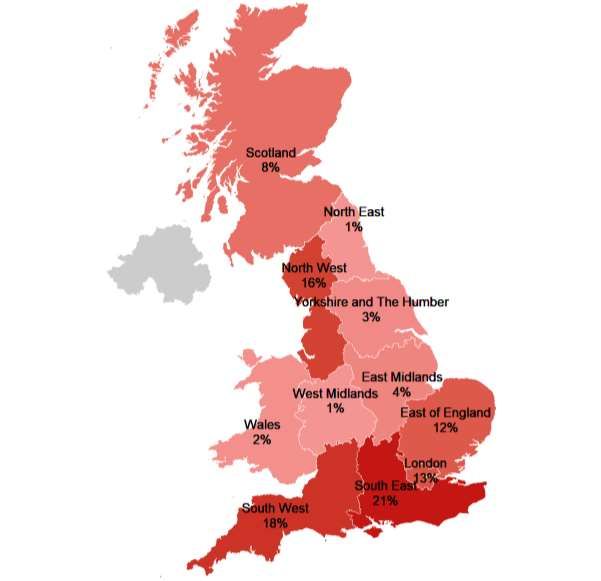
REVENUE AND
DISTRIBUTIONAL MODELLING
   FOR A UK WEALTH TAX
Arun Advani, University of Warwick, CAGE, the Institute for Fiscal Studies (IFS), and the LSE
International Inequalities Institute (III)

Helen Hughson, London School of Economics III

Hannah Tarrant, London School of Economics III

Wealth Tax Commission Evidence Paper no. 13

Published by the Wealth Tax Commission

www.ukwealth.tax

Contact    details:   Arun    Advani      (a.advani.1@warwick.ac.uk),     Helen     Hughson
(h.m.hughson@lse.ac.uk), Hannah Tarrant (h.l.thompson@lse.ac.uk)

Acknowledgements
The authors thank Andy Summers, Emma Chamberlain, David Burgherr, Daniel Butler, John
Barnett, and Edward Troup for helpful comments. The authors are also grateful to staff at
HMRC, HMT, ONS, and the VOA for providing information that served as input to the analysis.
The authors also thank Shaun Fu, Louis Goddard, Sam Leon, and Aruna Popescu for assistance
matching companies house data to the Sunday Times Rich List. This does not signify any
endorsement or agreement by any of the above of the conclusions in this paper.

This work contains statistical data from ONS which is Crown Copyright. The use of the ONS
statistical data in this work does not imply the endorsement of the ONS in relation to the
interpretation or analysis of the statistical data. This work uses research datasets which may not
exactly reproduce National Statistics aggregates.

The Wealth Tax Commission acknowledges funding from the Economic and Social Research
Council (ESRC) through the CAGE at Warwick (ES/L011719/1) and a COVID-19 Rapid
Response Grant (ES/V012657/1), and a grant from Atlantic Fellows for Social and Economic
Equity's COVID-19 Rapid Response Fund.

2
Abstract
In this paper we model the revenue that could be raised from an annual and a one-off wealth tax
of the design recommended by Advani, Chamberlain and Summers (2020b). We examine the
distributional effects of the tax, both in terms of wealth and other characteristics. We also
estimate the share of taxpayers who would face liquidity constraints in meeting their tax
liability. We find that an annual wealth tax charging 0.17% on wealth above £500,000 could
generate £10 billion in revenue, before administrative costs. Alternatively, a one-off tax
charging 4.8% (effectively 0.95% per year, paid over a five-year period) on wealth above the
same threshold, would generate £250 billion in revenue. To put our revenue estimates into
context, we present revenue estimates and costings for some commonly-proposed reforms to
the existing set of taxes on capital.

3
1. Introduction
The Wealth Tax Commission studied the possibility of a wealth tax for the UK (Advani,
Chamberlain and Summers, 2020a,b), and delivered a body of research into the desirability and
deliverability of such a tax. A crucial aspect for politicians in deciding whether or not to support
a tax on wealth is how much revenue it could raise. Meanwhile, public support will hinge at least
partly on how much people could be asked to pay.

In this paper we model the revenue that could be raised from an annual and a one-off wealth tax.
We first consider an annual wealth tax, and calculate the tax rates that would be needed to raise
£10 billion in revenue at various possible thresholds, taking into account likely behavioural
effects. We analyse the distributional effect of these tax structures in terms of who pays and
how much, both across the wealth distribution and across other characteristics. We also analyse
who is likely to face liquidity constraints. For some of these tax structures, we look at how the
revenue raised compares to the administrative burden, both for the government and the
taxpayer.

We find that a wealth tax could raise a substantial amount of revenue at relatively modest tax
rates. For an annual wealth tax, a flat tax of 0.17% on wealth above £500,000 could generate
£10 billion in revenue, but at a (proportionally) high ongoing administrative (admin) cost to
government of £1.2 billion. The admin costs to taxpayers are even higher, at £7.8 billion per year,
increasing substantially the effective tax rate inclusive of all taxpayer costs. At higher
thresholds, higher tax rates are required to generate a similar amount of revenue, but aggregate
admin costs are lower as there would be fewer taxpayers. For example, at £2 million the ongoing
admin costs to government fall to only 1% of the revenue raised, comparable with other major
taxes (HMRC, 2019). However, with a £10 billion revenue target, costs to the taxpayer amount
to a quarter of revenue raised. This effectively adds a cost of 0.13% of wealth to the headline
rate.

We then consider a one-off wealth tax. Since this is a one-off event, certainly not something that
would be seen for at least another generation, we consider the tax rate needed to raise £250
billion: the equivalent of raising an effective annual revenue of £10 billion per year over a 25-
year period. We also consider a flat rate of 1% a year for five years, as an alternative benchmark.
We perform an analogous set of analyses, studying distributional effects, liquidity constraints
and admin costs.

We find that a one-off wealth tax charging a tax rate of 4.8% on wealth above £500,000 would
generate £250 billion in revenue, before admin costs. This would come at a total cost of £1.7
billion to the government, and £7.8 billion to the taxpayer. Since this is a one-off event, it is
possible to achieve a much higher ratio of revenue to cost than under an annual wealth tax. A
higher threshold would reduce the admin cost further, though achieving the same amount of
revenue would necessitate higher rates. We estimate that with a threshold of £1 million, a one-
off tax of 8.5% – or a five-year annualised rate of 1.7% – would be required to raise £250 billion.
Under this tax structure, the cost to the government would be 0.4% of the revenue raised.
Taxpayer costs would be 1.8% of revenue raised, effectively adding a further 0.14% to the
headline rate.

Under a one-off wealth tax with an exemption threshold of £500,000 generating £250 billion in
revenue, we estimate that 6.4% of individuals would face liquidity constraints. This rises to 25%
with a threshold of £2 million, though the absolute number of liquidity constrained taxpayers
would fall, from 526,000 to 154,000. Fewer taxpayers would be liquidity constrained under an
annual wealth tax generating £10 billion in revenue.

4
Finally, we compare the revenue we could get from a wealth tax with the revenue that might be
raised by alternative reforms to the taxation of capital: in particular reforms to Capital Gains
Tax (CGT), taxation on dividend income, Inheritance Tax (IHT), and Council Tax. Numerous
reforms to these taxes have been proposed in recent years (APPG, 2020; Adam, Hodge, Phillips
and Xu, 2020; Corlett, 2018; Roberts et al., 2018). We focus on a few headline reforms that are
common to almost all reform proposals.

A brief comparison shows that it would be possible to raise similar amounts of revenue to an
annual wealth tax, or more, through some of the proposed reforms we examine. For example,
raising tax rates on capital gains to be in line with those on income would raise an additional £12
billion, with little implied cost to tax authorities, and equalising rates on dividends would raise
around £5 billion. On the other hand, a reform such as revaluing housing assets (and reforming
rates) for Council Tax could raise even more substantial amounts, for around half the one-off
cost to the government of implementing an annual wealth tax. These alternative reforms do not
necessarily avoid some of the challenges inherent in implementing a wealth tax, such as the cost
and difficulty of valuing assets.

The remainder of the paper is organised as follows. Section 2 describes the data we use and
adjustments we make to better capture wealth held at the top. Section 3 presents our revenue
modelling for an annual wealth tax, who would pay it, and how many taxpayers would face
liquidity constraints. We also discuss the effect of banding on our revenue estimates. Section 4
presents similar analysis to Section 3, this time for a one-off tax on wealth. Section 5 provides a
brief analysis of the revenue that could be raised from alternative reforms to the current tax
system. Section 6 concludes.

5
2. Data and Methods
2.1 Data
Wealth and Assets Survey
Our primary data source is the Office for National Statistics’ (ONS) Wealth and Assets Survey
(WAS), which is the most comprehensive data source on wealth in the UK. We use the most
recent wave of the data, collected in 2016–18, which covers around 40,000 individuals. The data
exclude certain geographical regions, in particular Northern Ireland, and the area north of the
Caledonian Canal. Individuals living in institutional settings, such as care homes, halls of
residence, and prisons, are also beyond the scope of the survey. As a result, we miss around 2%
of the UK population.

The WAS collects information on all major asset classes, including pensions, property, physical
wealth (consumer durables), financial wealth, and business assets, as well as liabilities.
Consumer durables are not included in the UK National Balance Sheet, which is constructed
following the System of National Accounts. However, physical assets such as vehicles, art
collections, antiques etc. are important household assets, and can be significant stores of value
for individuals at the top of the wealth distribution. We therefore include these assets in our
wealth definition. To construct a measure of 'net wealth', we deduct the value of loans including
mortgages, consumer loans, outstanding balances on credit cards and store cards, outstanding
balances on hire purchase agreements and mail order purchases, arrears on household bills and
loans, and current account overdrafts. We use this net wealth concept to calculate an
individual's tax liability.

In principle, we would like to include in our definition of tax-deductible loans any loan that has
been made legally binding, including formal loans between family and friends. Informal loans for
which there is no legal contract could be used for tax avoidance purposes if they are not tax
deductible. However, in practice such loans cannot be distinguished from gifts, and we do not
consider it feasible to include them in the tax base. Unfortunately, the WAS does not distinguish
between inter-household loans that have a formal legal contract, and those that do not. In our
main measure of taxable net wealth, we do not deduct 'loans from a friend, relative, or other
private individual' from an individual's gross wealth, effectively treating them all as informal.
Similarly, we exclude money loaned to other individuals from an individual's financial assets. The
revenue effect of excluding these informal loans is insignificant - in the tens of millions for a one-
off wealth tax raising £250 billion in revenue.

For our purposes, the valuation concept of interest is market value – the amount for which
assets could be sold. The WAS measures all assets that are relevant to our definition of the tax
base at market value. The exception is household contents, which we address in detail below.
These are recorded at replacement cost, which is likely to be significantly higher than the
amount for which household items could be sold second hand.

Our revenue modelling assumes a comprehensive tax base, covering each of these asset classes,
net of debts. Advani, Chamberlain and Summers (2020b) argue, however, that a wealth tax may
need to allow exemptions for low-value assets, and suggest a £3000 exemption per item. We
aim to define chargeable wealth – wealth that could be taxed – to be consistent with this. It is
not possible to model this precisely using the WAS, as wealth is not reported item-by-item, so
we make some necessary approximations.

6
For physical wealth, we start by excluding the value of all household contents. The questionnaire
is structured such that collectibles and valuables are asked about before the value of any other
household contents. Respondents are then instructed to "include all items, such as appliances
and electronic equipment, furniture, clothing and leisure items (but exclude any vehicles or
collectibles and valuables that you have already told me about)". Items worth more than £3000
are likely to have already been included under collectibles and valuables. However, it is possible
that some larger appliances and items of furniture would be worth more than £3000. To
examine the likelihood of this, we analyse eBay sales data to obtain the average sale price of new
and used household items, where we think of the new price as a proxy for replacement cost, and
the used price a proxy for market value. Table F1 shows the average price for a range of
narrowly-defined household items which might be included under the WAS household contents
category. All items are worth far less than £3,000 on average, even when new, and very few
items sell for more than £3,000. We interpret this as evidence that the majority of household
contents will be exempt from the wealth tax. In Appendix F, we show that the revenue effects of
including household contents are small, primarily because these assets are concentrated at the
bottom of the wealth distribution. This is important, as it suggests that the revenue implications
of taxing these assets will be small relative to the hassle cost of valuing them.

For categories likely to include items worth more than £3000, such as collectables and
valuables, vehicles, and personalised number plates, we exclude this wealth only if the total
amount reported in that category is less than £3000. We apply the latter rule to property wealth
(treating each category separately),1 and business assets (treating each business separately).
For pensions, we apply the £3000 rule to the category as a whole. We deduct the full value of
any debts. We do not allow an exemption on financial assets, as it is unlikely that such a rule
would be implemented in reality.

We use individual-level, rather than household-level data, to be consistent with the
recommendation of individuals as the tax unit in Advani, Chamberlain and Summers (2020b).
Most of the wealth recorded in the WAS is captured at individual level. For wealth recorded at
household level, which includes the main residence and certain categories of physical wealth
such as household contents, we divide the wealth equally between the head of household and
their partner, where applicable.

For our liquidity analysis, we use the concept of 'net income' as captured in the WAS, which is
measured at the individual level. This includes income from employment, self-employment,
state benefits, occupational and private pensions, investment income, and other regular income
(such as from friends and family, maintenance, royalties, overseas pensions, and rent), net of any
tax and National Insurance contributions paid by the individual. This income concept is broader
than fiscal income, which only captures income that is assessable for tax. It is less comprehensive
than income as recorded in the national accounts, which also includes income flows not directly
received by individuals, such as the imputed rent of owner-occupiers and investment income
received by pension funds. For the purpose of analysing liquidity constraints, it is important to
consider income flows which an individual could use in practice to fund wealth tax payments.
Including income flows such as imputed rents would understate the liquidity issues faced by
those living in valuable residential properties, for example. The income definition we use is
consistent with the liquidity analysis presented in Loutzenhiser and Mann (2021).

1
  Property wealth is divided into main residence, second homes, buy to let property, other buildings, UK
land, overseas land, overseas property, and other.
7
Sunday Times Rich List
A key caveat to relying on the survey data alone is that they under-represent wealth held at the
very top of the distribution. In response to this, we follow the approach set out in detail in
Advani, Bangham and Leslie (2021), which supplements the WAS with information from the
Sunday Times Rich List (STRL). We make a few adjustments to this methodology, as described
below.

The STRL captures, in theory, the 1000 richest people or families in Britain. The compilation and
measurement of wealth held by rich list individuals draws heavily on their observable business
assets. More private forms of wealth, such as financial assets, are generally not captured. We
proceed under the assumption that the wealth captured primarily reflects business wealth, and
that the total wealth recorded is likely to be an underestimate of the wealth held by these
individuals.

Though there are 1000 entries in the STRL, some entries include multiple individuals, such as a
husband and wife or other members of the same family. To be consistent with our use of
individual-level data in the WAS, we treat each individual named in the STRL as a separate unit.
Where there are multiple named individuals per rich list entry, we divide wealth equally among
them.

In contrast to Advani, Bangham, and Leslie (2021), we use data from the 2020 STRL. We rescale
this to match the aggregate wealth in the 2017 and 2018 (average of the two) lists, to be
consistent with the time period in which the WAS data were collected. Our reason for doing this
is to leverage information on the country of residence of STRL individuals, which we obtain using
matched records from Companies House. Individuals need not have the UK as their main
country of residence to be included in the STRL, and it is not clear that all individuals would
qualify as resident for tax purposes. This is important for our revenue analysis, as we seek to
establish how much revenue could be raised from those who are likely to be eligible to pay.

Though tax residence is not a readily observable characteristic, we can proxy for this using
information on country of residence as recorded in the Companies House register. Most
individuals in the STRL own or control part of a company registered with Companies House, and
these companies are required to submit information on their directors or ‘persons with
significant control’, including information on their usual country of residence.2 We have
matched individuals named in the STRL to Companies House records, using name and date of
birth as our matching criteria. We were able to match 83% of the 1,242 named individuals
automatically. A further 149 were matched manually, having been missed often as a result of
different variants of their name being used across the two data sources. For the remaining
unmatched 5% of individuals, we impute information on their country of residence based on the
percentage of individuals in each five-percentile bin of the STRL who are UK resident. In total,
we classify 84% of individuals as UK resident, although they make up only 74% of the wealth in
the STRL.

2.2 Pareto Imputation
We account for wealth missing from the top of the distribution in two ways. First, we add
individuals in the STRL to our WAS data, removing the handful of individuals whose wealth
overlaps with the STRL to ensure they are not accounted for twice. Second, as in Advani,

2
  A 'person with significant control' is usually someone who (a) owns more than 25% of shares in the
company; (b) holds more than 25% of voting rights in the company; or (c) holds the right to appoint or
remove the majority of the board of directors.
8
Bangham, and Leslie (2021), we implement a Pareto adjustment to estimate the amount of
additional wealth that should be captured in the top tail of the wealth distribution. The first step
increases our estimate of total wealth from £14.2 trillion to £14.6 trillion. The second step
increases this to £14.8 trillion.

It is widely observed that the top tail of the wealth distribution approximates a Pareto
distribution (e.g. Jones, 2015). By fitting a Pareto distribution using data on wealthy individuals
in the WAS combined with the STRL, we estimate the amount of excess wealth that is implied by
the shape of the distribution. We refer the reader to Advani, Bangham and Leslie (2021) for full
details of this approach.

We implement our Pareto adjustment to the distribution of business wealth (including shares),
rather than using total wealth as recorded in the WAS. This is to ensure consistency with what
is captured in the STRL, which we believe to be primarily business wealth. We choose a relatively
low threshold of £500,000 in business wealth, though in practice the chosen threshold has little
impact on the amount of additional wealth estimated. Using this approach, we estimate that
there is an additional £280 billion in wealth in excess of the wealth recorded in the WAS and the
STRL. This differs from the estimate in Advani, Bangham and Leslie (2020) for two reasons. First,
their paper uses household, rather than individual-level data to implement the Pareto
adjustment. Second, they assign each entry in the rich list a single household weight of 1,
whereas we assume each entry represents the number of individuals explicitly named in the rich
list.

To estimate the amount of revenue that could be raised from individuals across the wealth
distribution, we must allocate this additional Pareto wealth to observations in our data. We do
this by assigning to each individual in our Pareto sample the amount of business wealth they
would be expected to have according to their rank in the distribution. We then redefine each
individual’s total market value wealth, and total chargeable wealth, replacing their reported
business wealth with the amount implied by the Pareto distribution.

For the purpose of analysing liquidity issues, it is essential to know how an individual’s
chargeable wealth compares to their income. However, by adjusting wealth at the top of the
distribution, we have distorted this relationship. It is not clear how one could model a top wealth
or income adjustment that accurately captures the relationship between these two variables at
an individual level. Moreover, we do not wish to overstate the extent of liquidity issues by
assuming that wealth has been under-reported while income is accurately captured. As a result,
we have chosen to preserve the ratio of wealth to income as it is reported in the survey. We do
this by scaling net income by the ratio of an individual’s adjusted to unadjusted wealth. At an
individual level, the ratio of wealth to net income is therefore consistent with the liquidity
analysis undertaken in Loutzenhiser and Mann (2021). This adjustment makes very little
difference to our estimates: under each of our proposed tax structures, the percentage of
taxpayers deemed to be liquidity constrained is within half a percentage point of the result
obtained when reported income is used.

In our revenue analysis, we use the WAS data augmented with the STRL and our Pareto
adjustment. They are also included in our analysis of the distribution of taxpayers by age and
sex. However, we do not have information on their income, asset composition, or region of
residence. STRL individuals are therefore excluded from our analysis of the distribution of
taxpayers by region, liquidity constraints, and the asset composition of taxpayers.

9
3. Modelling an annual wealth tax
3.1 Approach
We model a wealth tax that is consistent with the recommendations outlined in Advani,
Chamberlain and Summers (2020b) using the data on wealth above various thresholds
described in the previous section. Our tax covers all adult individuals. Children are not taxed as
separate tax units. Instead, their wealth is aggregated with the wealth of their parents. We
assume that, in practice, parents would be able to choose who their children's wealth is allocated
to, and would do so to minimise their joint tax liability. Accordingly, we allocate children’s’
wealth reported in the WAS to the lower wealth parent, splitting any excess equally. In this way,
we preserve the wealth ranking between parents.

Though data from the STRL are included in our analysis, in our main specification we exclude
individuals who are classified as non-residents according to their Companies House records,
targeting tax residence as the relevant connection criterion.

We also take into account behavioural responses. As outlined in Advani and Tarrant (2021), a
net wealth tax is likely to elicit a number of avoidance and evasion responses, including under-
reporting, offshore evasion, gifting and fragmentation, asset portfolio recomposition, saving
responses, labour supply responses, and migration. Advani and Tarrant (2021) conclude that
under a well-designed wealth tax covering all asset classes – as we assume ours will – the overall
magnitude of behavioural responses could be limited to a 7–17% reduction in wealth in
response to a 1% tax rate on wealth. In our revenue modelling, we take the upper bound as the
‘high avoidance’ scenario, and the lower bound as the ‘low avoidance’ scenario. We apply this
response to the average tax rate faced by each individual under each tax structure. For example,
for an individual facing an average tax rate of 0.5%, we reduce their chargeable wealth by 3.5%
in the low avoidance scenario.

The figures 7% and 17% represent average behavioural responses, summarising the combined
effect of each individual’s response along the different margins. By applying this statistic in the
way we do, we will miss heterogeneity in avoidance responses across individuals. In practice,
some individuals will respond much more than others, and they will respond along different
margins. For example, these statistics partly reflect migration responses. Rather than modelling
who will choose to migrate and who will stay, we attribute the reduction in aggregate wealth
arising from some migration, to a reduction in the wealth of all individuals. In doing so, we
assume that behavioural responses are uniformly distributed across the wealth distribution.
While this may not hold in practice, we currently have very little empirical evidence on the
distribution of behavioural responses to a wealth tax (Advani and Tarrant, 2021). If the wealth
tax were at a flat rate (above some threshold), any heterogeneity would not affect our revenue
estimates. If the tax were progressive, our revenue estimates could be affected; however, in the
absence of information on how behavioural responses are distributed, it is not possible to even
sign the direction of the effect. In our distributional analysis, we focus on who should pay the tax,
and how much they should pay, rather than the amount they would pay after taking behavioural
responses into account. This will be unaffected by our method of accounting for behavioural
response in our revenue calculations.

Using household-level data we can explicitly model the potential revenue effects of asset
splitting between spouses. In addition to our core revenue estimates, which account for
avoidance using the elasticities provided in Advani and Tarrant (2021), we estimate the amount
of revenue that would be raised if all assets excluding pensions were split equally among the
head of household and their spouse. We do not split pensions, since these cannot typically be

10
transferred across individuals. We compare this to the revenue that would be raised if
ownership among spouses were unaffected by the introduction of a wealth tax. In doing so, we
assume no other avoidance responses. This is because our overall estimate of 7-17% already
accounts for asset splitting, and it is unclear what proportion of this average elasticity can be
attributed to asset splitting relative to other responses.

To calculate net revenue, we estimate the admin costs that the taxpayer and the tax authority
would face on an ongoing basis. Admin costs to the taxpayer partly reflect the valuation costs to
taxpayers which are likely to need professional valuations for their asset portfolios. A range of
cost estimates are calculated in Daly, Hughson, and Loutzenhiser (2021); here we estimate a
‘central’ scenario based on valuation costs amounting to 0.4% of the value of hard-to-value
assets (with the same overall cap).

Evidence presented by Burgherr (2021) suggests that there is also a fixed cost of filing which,
while generally dwarfed by the valuation cost, should be accounted for. We add a £2000 cost
for all taxpayers with hard-to-value assets, reflecting a central estimate from the range he
establishes; we do not attempt to account for the opportunity cost of the taxpayer’s time for
those taxpayers who (we assume) do their own filing. These estimates also do not attempt to
account for legal costs of disputes with the tax authority, as the scale and variation of these costs
are much less predictable. The valuation cost estimates cover a single year of a tax and do not
depend on the tax rate, nor do they vary between a one-off tax and an annual tax; in an annual
tax scenario with valuation only necessary every few years, costs could be expected to be lower
after the initial valuation.

We also calculate the one-off costs that the tax authority would incur in order to administrate
the tax. Our ongoing admin costs are based on the cost to HMRC of auditing Self Assessment
(SA) income tax returns. A wealth tax would be administered in much the same fashion, with
potential taxpayers having to submit a tax return, a certain percentage of which would be
audited by the tax authority. We assume that the cost of auditing a wealth tax return will be the
same as the cost of auditing a SA return, which is approximately £2,500 per audit (Advani,
Elming and Shaw, forthcoming). We will assume that 5% of wealth tax returns are audited,
suggesting that the average cost per tax unit to HMRC from auditing is around £125. To
calculate the total ongoing admin cost for each tax structure, we multiply this figure by the
number of filers, assuming that anyone who thinks they are within 10% of the tax threshold also
has to file a tax return. This means that the population of returns that could potentially be
audited will be slightly higher than the number of taxpayers.

There are two types of one-off cost we consider. First, the cost of revaluing residential property,
which we assume is done centrally rather than by the taxpayer, as is the case for Council Tax.
Second, the cost of designing and developing an IT system for administering the tax.

For the cost of revaluing residential property, we draw on the estimated cost of revaluating
properties for Council Tax in England, a project which began in 2001 but was never completed.3
In 2005 it was estimated that the revaluation would cost the Valuation Office Agency (VOA),
which was tasked with conducting the revaluation, £139.3 million in total.4 An additional £38
million was expected to be incurred in the first year from the cost of appeals. At this point, £45

3
  The revaluation exercise was due to be completed in April 2007 and would have been the first
revaluation since 1991. However, the exercise was postponed until it could happen ‘…as part of a fully
developed package of funding reforms, rather than as a precursor to them, and at a moment of greater
financial stability for local authorities’ (House of Commons Library Research Paper, 2005).
4
  House of Commons Library Research Paper 05/73, ‘The Council Tax (New Valuation Lists for England)
Bill’ (November, 2005).
11
million had already been spent on bringing the VOA’s systems up to date and digitising
documents of paper records, an exercise which would not need fully repeating if the revaluation
were resumed. Since these old documents may now partly be out-of-date, we take a
conservative approach by assuming that this cost would again be incurred in full. On this basis,
the exercise would have cost £180 million according to estimates from 2005. Scaling this to
2018 (the final year in our wealth tax data) by the rate of wage inflation, the most relevant cost
here, suggests that a present-day valuation would cost approximately £245 million.

We assume that this £245 million would be the cost of revaluing the entire housing stock. It is
possible that some fraction of this cost would be avoided, as not all properties would need to be
valued under a wealth tax with an exemption threshold. However, we do not know what this
fraction would be. Moreover, valuing properties at the top end of the property distribution is
likely to be much more costly than valuing a standard semi-detached house, and so we cannot
assume that the cost of revaluing the housing stock is proportional to the number of houses
valued. This is certainly not the case, as there will be fixed costs in producing a model for
estimating house values which would serve as the primary basis of valuation for the majority of
properties. Our cost estimate should therefore be thought of as an upper bound.

As a proxy for the cost of building a new system for administering the tax, we take the cost of
designing and developing the Customs Declaration Service, a system which went live in 2018.
The system will ultimately process over 250 million customs declarations, calculating the tariffs
due on each. The most recent estimate of the total cost of the project is £334 million. 5 This is a
comprehensive estimate which includes the cost of planning, designing, construction and
delivery, as well as ongoing maintenance costs.

3.2 Revenue
In this section we present estimates of combinations of rates and thresholds which would raise
£10 billion in tax revenue under a low avoidance scenario, before accounting for admin costs
(Table 1). This revenue target is not chosen to in any way be optimal, or reflect any kind of
recommendation. Instead it is selected as a useful benchmark, being roughly equivalent to
increasing the basic rate of income tax by 2p (HMRC, 2020a).

With a threshold of £10 million, a tax charged at 1.1% would raise £10 billion under a low
avoidance scenario, or £8.8 billion with high avoidance. Ongoing admin costs to government
here are essentially negligible, although there is some setup cost that is needed.

Lowering the threshold to £2 million, the same amount could be collected with a tax rate of just
0.57% under a low avoidance scenario. Now the number of taxpayers is substantially higher,
increasing from 22,000 to 631,000. The aggregate admin costs of the tax would be much higher
– the cost being largely borne by the taxpayer rather than the government.6 Costs to the
taxpayer amount to a quarter of revenue raised, effectively adding a cost of 0.13% of taxable
wealth to the headline rate.7

5
  HMRC Government Major Project Portfolio data, September 2019.
6
  Note that for purposes of Total Managed Expenditure calculations, the admin cost to government can
likely be reduced by around one-third, since these costs are largely salaries, and one third of this cost will
be returned to the exchequer in income tax and national insurance contributions. However, the full value
of the cost must be taken into account when considering the efficiency of the tax.
7
  This figure is calculated by dividing the aggregate admin cost to taxpayers by aggregate wealth above
the threshold, before taking avoidance into account.

12
At 22,000 taxpayers, the volume of taxpayers under an annual wealth tax beginning at £10
million is similar to IHT (which covers 24,000 taxpayers per year). Comparable amounts could
be raised with a progressive tax, covering the same number of taxpayers but at lower rates for
those with less wealth, as shown in one particular example in the final row of Table 1.

With a threshold of £500,000, 8% of the revenue raised comes from individuals in the STRL.
The importance this group becomes more pronounced the higher the threshold: with a
threshold of £5 million, these individuals account for 40% of our revenue estimate. This
reflects the concentration of wealth at the very top.

13
TABLE 1: REVENUE ESTIMATES FOR AN ANNUAL WEALTH TAX – FLAT AND PROGRESSIVE TAXE
Revenue (£bn) Administrative cost (£bn): Share of
revenue
Threshold Low High Taxpayers one-off per year from
to taxpayer
(£) Rate avoidance avoidance ('000) to govt to govt STRL
Flat taxes
1.12
10,000,000 % 10.0 8.8 22 0.7 0.6 0.003 50%
0.90
5,000,000 % 10.0 9.0 83 1.4 0.6 0.01 40%
0.57
2,000,000 % 10.0 9.4 631 2.5 0.6 0.1 25%
0.31
1,000,000 % 10.0 9.7 3,035 4.6 0.6 0.5 14%
0.17
500,000 % 10.0 9.8 8,240 7.8 0.6 1.2 8%
0.12
250,000 % 10.0 9.9 15,537 10.7 0.6 2 5%
Progressive taxes
0.10
1,000,000 %
0.25
2,000,000 %
10.0 9.5 3,035 4.6 0.6 0.1 29%
0.50
5,000,000 %
0.65
10,000,000 %
Notes: The rates target £10bn in revenue, taking into account a low level of avoidance, and before the deduction of
admin costs.
Source: ONS, Wealth and Assets Survey, 2016–18; Sunday Times Rich List, 2020; Burgherr, 2021; Daly, Hughson,
and Loutzenhiser, 2021; House of Commons Library, 2005; HMRC Government Major Project Portfolio data, 2020d.
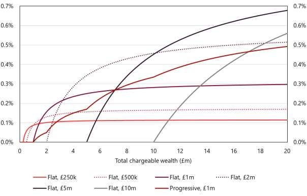
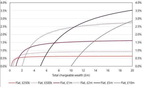
The amount of revenue raised by a tax with a given threshold can be varied by changing the
rates. Figure 1 illustrates the rates that would be required to raise different revenue targets, net
of ongoing admin costs to government. Evidently, the rates required to generate a given amount
of revenue at a given threshold are higher when individuals are more responsive to the tax.
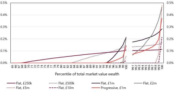
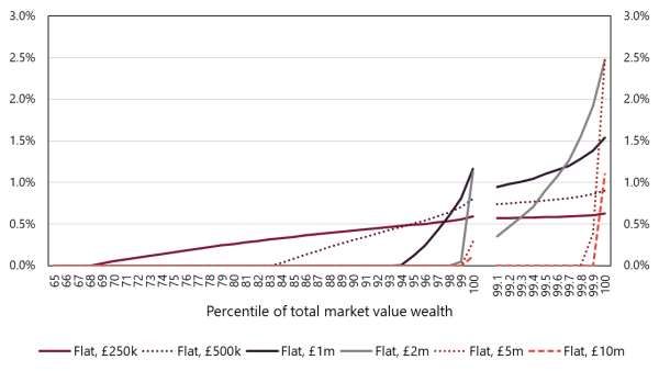
14FIGURE 1: RATES AND THRESHOLDS GENERATING DIFFERENT REVENUE TARGETS FROM AN ANNUAL WEALTH TAX, AFTER ADMIN COSTS Notes: Tax rates are those required to generate the revenue target after admin costs are taken into account. Source: ONS, Wealth and Assets Survey, 2016–18; Sunday Times Rich List, 2020. To understand the potential revenue effects from asset splitting, we model the revenue that would be raised if all assets, other than pensions, were split equally between the household head and his/her partner. Using the headline rates presented in Table 1, we first estimate the revenue that could be raised if assets were retained by the household member who owns them currently (Table G1). In the absence of any avoidance responses, revenue would be up to £0.9 billion higher than in our low avoidance scenario. However, if households were to respond to the tax by splitting their assets equally, revenue would be reduced by 1-7% (up to £0.7 billion). Note that this revenue loss is smaller than the revenue loss obtained by moving to our 'low avoidance' scenario. Our 'low avoidance' measure is intended to be comprehensive of the range of behavioural responses available to individuals. It is reassuring to find that the revenue loss from asset splitting – even when modelled to the extreme – is lower than our more optimistic measure of avoidance responses, particularly as asset shifting is a known response to individual taxation (Advani and Tarrant, 2021). 3.3 Distributional Effects If the UK were to introduce an annual wealth tax, who would pay it? And how would the amount of tax paid vary across individuals? In this section, we explore how tax liabilities would vary across the distribution of income and wealth under each of the annual tax structures presented in Table 1, assuming the rates required to generate £10 billion before admin costs under a low avoidance scenario. We then consider the characteristics of taxpayers, specifically considering age, sex, and region. We include individuals in the STRL when looking at the distribution by wealth, age and sex. However, as we have no information on their income nor region of residence, this analysis is based on the WAS data only. Table 2 shows the amount of tax paid by a representative individual with different levels of wealth. A higher threshold does not necessarily mean that an individual who is still liable to pay the tax will face a smaller tax liability. Taking an individual with £7.5 million in wealth as an 15
example, the tax liability that this individual faces is £20,150 under a flat tax starting at £1
million. If the threshold rises to £2 million, the rate required to generate the same amount of
revenue as before means that the same individual would now face a tax liability of £31,350.
An exemption threshold of £250,000 would not charge any wealth tax to anyone in the bottom
70% of the wealth distribution. Nevertheless, by international standards this would be a very
low threshold: only Switzerland is lower (Chamberlain, 2020). With a relatively low exemption
threshold of £250,000, the average tax rate faced across the wealth distribution would increase
steadily, reaching 0.12% (equal to the marginal tax rate) for those in the top 1%. With a higher
exemption threshold, the average tax rate increases more rapidly. Individuals in the top 1%
would face an average tax rate of 0.21% with an exemption threshold of £2 million, for a tax
generating £10 billion in revenue (see Fig. 2).
TABLE 2: AMOUNT OF TAX PAID BY A REPRESENTATIVE INDIVIDUAL UNDER AN ANNUAL TAX WITH
DIFFERENT THRESHOLDS, (£)
Threshold (£) Rate Individual net wealth (£)
750,00 1,500,00 3,000,00 7,500,00 15,000,00
0 0 0 0 0
Flat taxes generating £10bn
1.12
10,000,000 % 56,000
0.90
5,000,000 % 22,500 90,000
0.57
2,000,000 % 5,700 31,350 74,100
0.31
1,000,000 % 1,550 6,200 20,150 16,800
0.17
500,000 % 425 1,700 4,250 11,900 24,650
0.12
250,000 % 600 1,500 3,300 8,700 17,700
Progressive taxes generating £10bn
0.10
1,000,000 %
0.25
2,000,000 %
500 3,500 21,000 66,000
0.50
5,000,000 %
0.65
10,000,000 %
Number of
individuals with
similar wealth
(within 10%),
thousands 1,508 573 107 14 5
Notes: Calculations of the tax liability of individuals at different points of the wealth distribution, under each tax
schedule shown in Table 1. 'Number of individuals with similar wealth' shows the number of individuals whose net
wealth is within 10% of the representative individual, giving a rough indication of the number of individuals who
would face that tax liability.
Source: ONS, Wealth and Assets Survey, 2016–18.
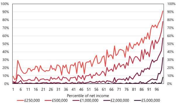
16FIGURE 2: MEAN AVERAGE TAX RATE UNDER DIFFERENT ANNUAL TAX STRUCTURES Notes: All adult individuals are ranked according to their total wealth measured at market value, and grouped into percentiles. Tax rates used are as per Table 1. The average tax rate faced by individual is the amount they should pay, and does not take behavioural responses into account. We take the democratic mean of average tax rates faced in each percentile. Appendix A shows the average tax rate by total chargeable wealth. Source: ONS, Wealth and Assets Survey, 2016–18; Sunday Times Rich List, 2020. On the whole, individuals higher up the income distribution are more likely to pay a wealth tax (Fig. 3). However, at each level of income there is some variation in wealth, and not all high- income individuals have sufficient wealth to become taxpayers. Among those in the top 1% of the income distribution, 91% would pay a wealth tax with an exemption threshold of £250,000, compared with 25% of the population. As the threshold rises to £2 million, 33% would be liable to pay, and at a threshold of £5 million this figure falls to just 8%. Meanwhile, among those at the median of the income distribution, 10% would be liable to pay a wealth tax with an exemption threshold of £500,000. 17
FIGURE 3: SHARE OF INDIVIDUALS WHO ARE TAXPAYERS UNDER DIFFERENT EXEMPTION THRESHOLDS,
BY INCOME PERCENTILE

Notes: All adult individuals are ranked according to their net income, and grouped into percentiles. The chart shows
the percentage of adults in each percentile group who would pay the tax for different exemption thresholds. The
distribution is independent of the rate chosen, for a given threshold. Individuals in the Sunday Times Rich List are
excluded from this analysis, as we have no information on their income. We do not show the distribution of taxpayers
for thresholds above £5 million due to small sample sizes.
Source: ONS, Wealth and Assets Survey, 2016–18.

Older age groups are significantly over-represented among taxpayers for every threshold
(Fig. 4). Despite accounting for just 39% of the adult population, adults over the age of 55
represent 60% of taxpayers when a £5 million threshold applies, rising to as much as 75% with
an exemption threshold of £2 million. This figure illustrates clearly that the majority of
taxpayers would actually be of working age, with those in the 55–64 age category being the
most heavily represented. Only 1–2% of taxpayers are under the age of 35.

The higher the threshold, the higher the percentage of taxpayers who are male (Fig. 5). For each
threshold, female taxpayers are in the minority. The gender imbalance is most pronounced
under a wealth tax starting at £5 million, under which 68% of taxpayers are male. Note that this
is assuming individuals do not adjust their wealth holdings in response to the tax. For a tax which
defines the tax unit as the individual, we might expect some asset shifting within couples as a
means of reducing their joint tax liability. This would make the gender imbalance less extreme
in practice.

18
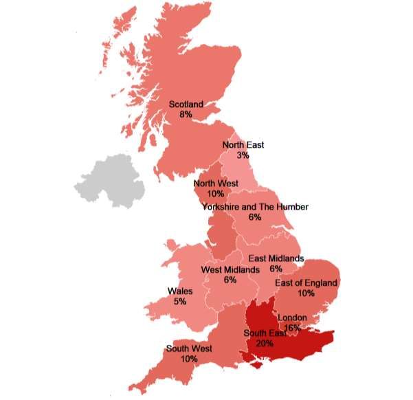
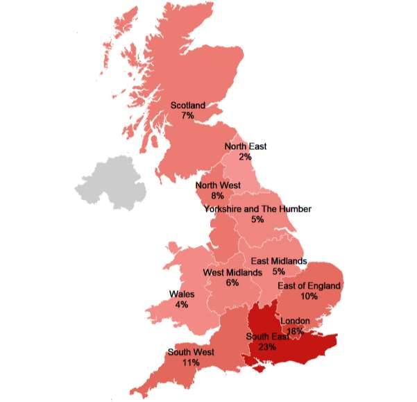
FIGURE 4: AGE DISTRIBUTION OF TAXPAYERS UNDER DIFFERENT EXEMPTION THRESHOLDS

Notes: The age distribution of taxpayers above different exemption thresholds is independent of the tax rate.
Individuals from the Sunday Times Rich List are included in this analysis.
Source: ONS, Wealth and Assets Survey, 2016–18; Sunday Times Rich List, 2020.

FIGURE 5: SEX DISTRIBUTION OF TAXPAYERS UNDER DIFFERENT EXEMPTION THRESHOLDS

Notes: The gender distribution of taxpayers above different exemption thresholds is independent of the tax rate.
Individuals from the Sunday Times Rich List are included in this analysis.
Source: ONS, Wealth and Assets Survey, 2016–18; Sunday Times Rich List, 2020.

The geographical distribution of prospective taxpayers is skewed toward London and the South
East, regardless of which threshold is chosen. Figure 6 illustrates the distribution of taxpayers
for a tax starting at £500,000, under which London and the South East combined would account

19
for 36% of all taxpayers.8 By contrast, just 3% of taxpayers live in the North East. The majority
of taxpayers live in England; Scotland and Wales account for just 12% of taxpayers. Appendix B
shows the geographical distribution of taxpayers for alternative exemption thresholds.

FIGURE 6: GEOGRAPHICAL DISTRIBUTION OF TAXPAYERS WITH A £500,000 EXEMPTION THRESHOLD

Notes: This chart shows how taxpayers would be distributed across the country if the tax featured an exemption
threshold of £500,000. The distribution is independent of the tax rate. Individuals in the Sunday Times Rich List are
not included in this analysis as we have no information on their region of residence. Appendix B shows the
geographical distribution of taxpayers using different exemption thresholds. We have no data for Northern Ireland,
and so the percentages shown are the percentage of taxpayers in Great Britain living in each region.
Source: ONS, Wealth and Assets Survey, 2016–18.

3.4 Liquidity Issues
Specific solutions may be required for individuals who face high tax liabilities relative to their
income, especially if much of their wealth is illiquid. In this section, we illustrate the extent of

8
    This is the percentage of taxpayers in Great Britain, as we do not have data for Northern Ireland.
20
liquidity problems faced by individuals under the annual tax structures presented in Section 3.2.
We ask how many individuals are liquidity constrained under each of the tax structures raising
£10 billion in revenue, and which groups of individuals are most affected.
In principle, we may define an individual as being liquidity constrained if, as a result of their
wealth tax liability, they would be forced to either reduce their consumption and standard of
living, or maintain their consumption by converting some of their illiquid wealth into cash.
However, in practice, we do not have a comprehensive dataset which captures income, wealth,
and expenditure at an individual level. Rather than combining multiple datasets to approximate
consumption levels at different points of the wealth distribution, we adopt a simpler approach.
For each tax schedule, we classify an individual as being liquidity constrained if their immediate
tax liability exceeds 20% of their net income and 10% of their net income plus liquid assets. In
Appendix C, we illustrate the extent of liquidity issues using alternative cut-offs, to show how
our estimates change when this definition becomes more or less generous.
We recognise that a specific solution is needed for the payment of taxes on pension wealth, as
individuals below State Pension Age (SPA) generally do not have access to these funds. As
recommended in Advani, Chamberlain and Summers (2020b), a solution to this would be to
allow individuals below SPA to pay any tax due on their pension wealth out of their lump sum
once they reach SPA. Accordingly, we assume that once an individual reaches SPA, all of their
wealth is ‘immediately taxable’. For individuals below the SPA, we define immediately taxable
wealth as all non-pension wealth, plus the value of pensions that are already in payment, as this
wealth has already been accessed.9
We define ‘liquid wealth’ as financial wealth, plus certain forms of pension wealth depending on
whether the individual is above or below SPA. If the individual is below SPA, we assume that all
of their pension wealth is illiquid.10 If the individual is above SPA, we assume that any remaining
wealth in a Defined Contribution pension pot becomes liquid, plus any lump sums from Defined
Benefit pensions that have not yet been claimed. However, wealth arising from the discounted
stream of income from a Defined Benefit or annuitised pension pot, or any other form of regular
pension income, is assumed to be illiquid. 11 In practice, it is difficult to distinguish between liquid
and illiquid forms of wealth. We expect some of our assumptions to classify too much pension
wealth as illiquid, but that our classification of all financial wealth as liquid will have the opposite
effect. It is not clear whether the net effect is positive or negative.
Of the annual tax structures raising £10 billion in revenue, a flat tax starting at £1 million
generates the largest number of liquidity constrained taxpayers, with over 48,000 taxpayers
facing liquidity issues (Fig. 7). Generally speaking, the lower the threshold, the lower the share
of taxpayers who are liquidity constrained. A flat tax starting at £250,000 generates 32,000
liquidity constrained taxpayers, representing just 0.2% of taxpayers (Fig. 8). By contrast, though
the number of liquidity constrained taxpayers is much lower for a tax starting at £5 million, at
17,000, this accounts for 20.3% of all taxpayers at this threshold. Note that for each tax
9
A 'pension in payment' is one from which an individual is receiving a regular income stream. It is possible
that there will be some individuals below SPA who have already accessed their pension pot, but are not
receiving a regular income from their pension. We expect this wealth to be immediately taxable, but are
unable to include these pensions in our definition of immediately taxable wealth due to data limitations.
10
It is possible that for individuals deriving a regular income from a pension, some of this wealth is in fact
liquid. This will not be the case for Defined Benefit payments or income from an annuity, but may be the
case if the income is being received through a flexible drawdown arrangement. It is not possible for us to
separate these income streams in order to classify them separately as liquid or illiquid, and so we treat all
pension in payment as illiquid. This applies to individuals both above and below SPA.
11
This includes Additional Voluntary Contribution pots that are part of Defined Benefit or hybrid
schemes. It also includes both personal and occupational pensions.
21structure, we are adjusting the tax rates to target £10 billion in revenue. Therefore, the higher
the threshold, the higher the marginal tax rate faced by individuals at the top. If we did not adjust
the rates, then raising the threshold would reduce the number of liquidity constrained
taxpayers, but this would also reduce revenue.
Under an annual wealth tax generating £10 billion before admin costs, the majority of liquidity
constrained taxpayers have a business as their main asset (Fig. 9). The lower the threshold, the
more evenly spread the composition of assets among those who are liquidity constrained. At a
threshold of £250,000, 14% of liquidity constrained taxpayers have their main residence as
their main asset. As the threshold rises to £1 million, this percentage falls to 4%. At higher
thresholds, business assets become much more important among those who are liquidity
constrained. At a threshold of £500,000, 57% have a business asset as their main asset. With a
threshold of £5 million, 94% have a business as their main asset.
FIGURE 7: NUMBER OF TAXPAYERS ('000) LIQUIDITY CONSTRAINED UNDER TAXES RAISING £10BN IN
REVENUE, BY RANGE OF NET WEALTH
Notes: An individual is liquidity constrained if their immediate tax liability (defined in Section 3.4) exceeds more than
20% of their net income and 10% of their net income plus liquid wealth. Tax rates used are as per Table 1. Individuals
in the Sunday Times Rich List are not included in this analysis. For individuals at the top of the WAS, we use their
Pareto-adjusted business wealth values, but adjust their net income to maintain the same ratio of wealth to income
as reported in the WAS. We do not present liquidity analysis using thresholds above £5 million due to small sample
sizes. The numbers underlying this graph are provided in Appendix C.
Source: ONS, Wealth and Assets Survey, 2016-18.
22FIGURE 8: PERCENTAGE OF TAXPAYERS LIQUIDITY CONSTRAINED UNDER TAXES RAISING £10BN IN REVENUE, BY RANGE OF NET WEALTH Notes: An individual is liquidity constrained if their immediate tax liability (defined in Section 3.4) exceeds more than 20% of their net income and 10% of their net income plus liquid wealth. Tax rates used are as per Table 1. Individuals in the Sunday Times Rich List are not included in this analysis. For individuals at the top of the WAS, we use their Pareto-adjusted business wealth values, but adjust their net income to maintain the same ratio of wealth to income as reported in the WAS. We do not present liquidity analysis using thresholds above £5 million due to small sample sizes. The numbers underlying this graph are provided in Appendix C. Source: ONS, Wealth and Assets Survey, 2016–18. FIGURE 9: MAIN ASSET AMONG THOSE WHO ARE LIQUIDITY CONSTRAINED UNDER DIFFERENT ANNUAL TAX STRUCTURES GENERATING £10BN IN REVENUE Notes: An individual’s main asset is the largest asset in their wealth portfolio after the exemption of low-value items (see Section 2.1 for details). Individuals in the Sunday Times Rich List are not included in this analysis. For individuals at the top of the WAS, we use their Pareto-adjusted business wealth values. We do not present liquidity analysis using thresholds above £5 million due to small sample sizes. Source: ONS, Wealth and Assets Survey, 2016–18. 23
3.5 Banding
Daly, Hughson and Loutzenhiser (2021) discuss in detail the challenges of establishing the exact
value of a person’s total wealth at a given point in time—a difficult exercise which is nonetheless
necessary for all taxpayers captured in the flat (or progressive) tax regimes described above.
One way to address this problem is to use a regime of tax bands, within each of which the tax
charge is a fixed fee: this will obviate the need for exact valuations of wealth for many
taxpayers.12 In this section we discuss how revenue raised changes if using a banded regime
rather than one of the flat tax regimes as discussed above.

Hughson (2020) addresses many of the issues and challenges in using such a regime as an
alternative to a flat or progressive tax as described above. A key insight from this work is that a
banding scheme is a blunt instrument which generates inequity: in a band covering wealth of
£1–£2 million, someone with £1 million in wealth pays the same amount in tax as someone with
almost twice as much wealth, and (perhaps substantially) more than someone with just under £1
million. There is a tension between limiting the extent of this inequity by setting bands narrow
enough to effectively target wealth, and setting them wide enough to materially simplify the
reporting burden of a significant proportion of taxpayers.

We demonstrate an example banding scheme with bands of increasing widths of total wealth:
£500,000–£1 million, £1–2 million, £2–4 million, £4–8 million, £8–16 million, £16–32 million,
and £32 million and over. We set the charge within bands based on the midpoint of the band
(multiplied by a rate of 0.17%, for comparability with a flat tax starting at £500,000).13 The
charge for the (open-ended) top of the band is set with reference to 150% of the threshold.

Figure 10 demonstrates what such a scheme would imply in terms of the effective average tax
rate (EATR) paid – that is, the relevant banding charge divided by an individual’s total wealth.
The amount of tax paid under the banded regime is equal to the flat tax (only) at the midpoint of
each band, and the band thresholds are clearly traced out at the points the EATRs jump higher.
The vertical inequality created is clear: those at the bottom of each band pay a larger share of
their wealth in tax than people at the top. The long tail at the right-hand side of the graph
demonstrates a difficulty plaguing any banding regime: because the wealth distribution has such
a long, thin tail, it is difficult to design a set of thresholds in which the very wealthiest members
of society pay anything other than a tiny proportion of their total wealth in tax (especially as
compared to others at the bottom of the same band, who may pay extremely high rates).

12
   The current Annual Tax on Enveloped Dwellings (ATED) regime functions in a similar way, although it
is only applied to one asset class (property).
13
   Hughson (2020) discusses in some detail the issues involved in the choice of the tax charge within each
band. A charge based on median wealth in the band would imply lower tax rates throughout and revenues
closer to the equivalent flat tax regime, but is more difficult to justify for wider and wider bands, as well
as being harder to implement in practice.
24
You can also read