Automated Theorem Proving 4/4: Satisfiability Checkers, SAT/SMT

Automated Theorem Proving 4/4:
     Satisfiability Checkers, SAT/SMT

                      A.L. Lamprecht

Course Program Semantics and Verfication 2020, Utrecht University

                    September 30, 2020

Lecture Notes

“Automated Reasoning” by Gerard A.W. Vreeswijk.
Available for download on the course website.
My slides are largely based on them.

In This Course

• Propositional theorem proving (last Monday),
  Chapter 2 of the lecture notes
• First-order theorem proving (last Wednesday),
  Chapter 3 of the lecture notes
• Clause sets and resolution (Monday),
  Chapters 4 and 5 of the lecture notes
• Satisfiability checkers, SAT/SMT (today),
  Chapter 6 of the lecture notes, additional material

Recap: Clause Sets and Resolution

• Conjunctive Normal Form (CNF)
• Clause sets
• Conversion to ≤3CNF in linear time (Tseitin-derivative)
• Cleaning up and simplifying clause sets (one-literal rule,
  monotone variable fixing, tautology rule, subsumption, DPLL)
• Binary resolution, linear/unit/input resolution
• Semantic resolution, ordered resolution, semantic clash,
  hyperresolution
• First-Order Resolution
• Normalization, Skolemization
• Equality, Demodulation, Paramodulation

Satisfiability Checkers

• Resolution can only be used to prove that a clause set is
  unsatisfiable.
• To be able to discover satisfiable formulas, we need
  satisfiability tests.
• Such tests try to find a satisfying assignment of φ.
• If such an assignment is found, the formula is proven
  satisfiable and the search can be stopped.
• Two popular satisfiability tests:
   1 Gradient of polynomial transforms of CNFs.
   2 Weighted variant of a greedy local search algorithm.

Gradient of Polynomial Transforms of
                                         CNFs

• Choose a proposition.
• Set to true if its number of unnegated occurrences is higher
  than its number of negated occurrences, otherwise set to false.
• Apply simplification rules.
• Repeat until a satisfiable assignments has been constructed.

Local Search

• Start with a random assignment of variables.
• Invert the truth values of a number of variables, so that the
  weight of satisfied clauses increases.
• If further inversion yields no improvement, the weights of the
  unsatisfied clauses are increased until an improving inversion
  comes into existence.
• Thus, “difficult” clauses receive large weights and are more
  likely to be satisfied in the end.
• Repeat until either a satisfiable assignment is constructed, or
  the number of inversions exceeds a certain maximum.
• For many satisfiable formulas the local search algorithm is
  sufficient for finding a model quickly.

GSAT

• Popular example of a local search algorithm.
• Given a clause set S, GSAT tries to find a model m such that
  m |= S by performing a greedy local search within the space
  of possible models.

GSAT (cont’d)

• GSAT only explores potential solutions that are close to the
  one currently being considered (differing only in one variable).
• Clearly, GSAT could fail to find an assignment even if one
  exists, i.e. it is incomplete.
• Specific feature of GSAT: Chooses at random the variable
  whose assignment is to be changed from those that would
  give an equally good improvement.
• Thus, unlikely that the algorithm makes the sequence of
  changes over and over.
• Another characteristic: GSAT makes sidesteps (flips variables
  without increasing the number of satisfied clauses).
• Thus, it can move over “plateaus” to get to better spots
  where improvements are again possible.

GSAT for Non-Clausal Formulas

  • GSAT can also be applied to non-clausal formulas.
  • To show how, we first define the criterion for satisfaction on
    clause sets:

Definition
The penalty of a model m on a clause set S, written pen(S, m), is
equal to the number of clauses in S that are made false by m.

  • Thus, the purpose of GSAT is to find a model m for S with
    penalty as low as possible.
  • In fact, pen(S, m) = 0 means m |= S.

GSAT for Non-Clausal Formulas (cont’d)

• GSAT works by considering proposition variables that, when
  flipped, bring the penalty down as much as possible.
• Write

     ∆(S, m, p) =Def pen(S, m with p flipped) − pen(S, m)

• GSAT tries to go downhill and searches for p in the direction
  where the slope ∆(S, m, p) is negative.

GSAT for Non-Clausal Formulas (cont’d)

• The penalty function pen may now be extended to a penalty
  function Pen on arbitrary formulas:
• For literals L, Pen(m, L) = pen(m, L), that is,
                                
                                    1 if m 2 L,
                  Pen(m, L) =
                                    0 otherwise.

GSAT for Non-Clausal Formulas (cont’d)
Further, Pen− (m, L) = 1 − pen(m, L), and

       Pen(m, ¬φ1 ) = Pen− (m, φ1 )
  Pen(m, φ1 ∧ φ2 ) = Pen(m, φ1 ) + Pen(m, φ2 )
  Pen(m, φ1 ∨ φ2 ) = Pen(m, φ1 ) · Pen(m, φ2 )
 Pen(m, φ1 ⊃ φ2 ) = Pen− (m, φ1 ) · Pen(m, φ2 )
 Pen(m, φ1 ≡ φ2 ) = Pen− (m, φ1 ) · Pen(m, φ2 ) + Pen(m, φ1 ) · Pen− (m, φ2 )

and

      Pen− (m, ¬φ1 ) = Pen(m, φ1 )
Pen− (m, φ1 ∧ φ2 ) = Pen(m, φ1 ) · Pen(m, φ2 )
Pen− (m, φ1 ∨ φ2 ) = Pen(m, φ1 ) + Pen(m, φ2 )
Pen− (m, φ1 ⊃ φ2 ) = Pen(m, φ1 ) + Pen− (m, φ2 )
Pen− (m, φ1 ≡ φ2 ) = (Pen(m, φ1 ) + Pen− (m, φ2 )) · (Pen− (m, φ1 ) + Pen(m, φ2 ))

GSAT for Non-Clausal Formulas (cont’d)

It can be proven that, for every arbitrary formula φ,

                  Pen(m, φ) = pen(m, CNF(φ))

where CNF(φ) is a CNF-conversion of φ.

Pen and Pen− can be computed in time linear to the length of φ.

So, plug in Pen into GSAT and apply GSAT to arbitrary formulas.
Result: NC-GSAT (very efficient implementations).

Shortcomings of GSAT

• GSAT often “wanders” through large plateaus of
  truth-assignments that show no variation.
• Can easily be misled into exploring the wrong part of the
  search space.
• Search is non-deterministic, so that trials are not reproducible.

Improvements of GSAT

• Random Walk Strategy (to escape from local minima):
    • With probability p, flip a variable that occurs in some
      unsatisfied clause.
    • With probability 1 − p, follow the standard GSAT scheme, i.e.,
      make the best possible local move.
  Upward moves (which would otherwise lead us astray) are now
  used to “repair” unsatisfied clauses.

Improvements of GSAT

• Random Walk Strategy (to escape from local minima):
    • With probability p, flip a variable that occurs in some
      unsatisfied clause.
    • With probability 1 − p, follow the standard GSAT scheme, i.e.,
      make the best possible local move.
  Upward moves (which would otherwise lead us astray) are now
  used to “repair” unsatisfied clauses.
• The WalkSAT algorithm takes this idea one step further and
  makes it the central component of the algorithm:
     • Randomly select an unsatisfied clause.
     • If the clause has a variable that can be flipped without
       breaking other clauses, that variable is flipped.
     • Else, with probability p we flip the variable that breaks the
       fewest clauses, and with probability 1 − p we flip a random
       variable in the selected clause.

Propositional Formula Checkers

Theorem proving amounts to verifying whether ψ follows from
φ1 , . . . , φn , for some φ1 , . . . , φn and ψ. There are two possibilities:
either φ1 , . . . , φn ` ψ or φ1 , . . . , φn 0 ψ.
  1   If “`”, then φ1 ∧ . . . ∧ φn ∧ ¬ψ is not satisfiable, which can be
      shown by means of a refutation method, such as resolution or
      the tableaux method.
  2   If “0”, then φ1 ∧ . . . ∧ φn ∧ ¬ψ is satisfiable and this can be
      proven by finding a countermodel.

Propositional Formula Checkers (cont’d)

• Satisfiability as well as unsatisfiability can be expressed by an
  existential statement.
• φ is satisfiable if there exists a satisfying assignment for φ.
• φ is unsatisfiable if there exists a refutation (resolution
  refutation or tableau refutation) of φ.
• In general, writing down a resolution proof is harder than
  writing down a satisfying assignment.
• This non-symmetry is caused by the fact that the satisfiability
  problem (aka SAT) is NP-complete, and propositional
  provability is co-NP-complete (see page 37 in the lecture
  notes).

Propositional Formula Checkers (cont’d)

• Still, resolution is the most powerful resolution method.
• State-of-the-art theorem provers are based on the
  manipulation of clause sets (not refutation trees).
• Tableaux method: search for a countermodel coincides with
  the search for a refutation.
• Thus, a tableaux is always useful.
• Not true for resolution refutation.
• Resolution can only prove (1), but never (2).
• To prove (2), so-called model-checking techniques are used
  (trying to guesss countermodels).

Propositional Formula Checkers (cont’d)

• A propositional formula checker (PFC) is an ATP program
  that is able to prove valid formulas, and disprove invalid
  formulas.
• Tableau method is “complete enough” to form the basis for a
  PFC, resolution is not.
• Resolution needs to be supplemented with some sort of model
  checking.

SAT/SMT

Here we leave the Vreeswijk lecture notes. The following slides are
based on mainly three sources:
  1   Dennis Yurichev’s “SAT/SMT by Example” (https:
      //yurichev.com/writings/SAT_SMT_by_example.pdf)
  2   The “Programming Z3” tutorial (https://theory.
      stanford.edu/~nikolaj/programmingz3.html)
  3   The paper “Satisfiability Modulo Theories: Introduction and
      Applications” by De Moura et al., available on the course
      website.

SAT/SMT

• SAT/SMT solvers deal with huge systems of equations.
• (A lot of real world problems can be represented as problems
  of solving system of equations.)
• Difference: SMT solvers take systems in arbitrary format,
  while SAT solvers are limited to boolean equations in CNF.
• SMT solvers are frontends to SAT solvers.
• Some SMT solvers use external SAT solvers (e.g. STP uses
  MiniSAT or CryptoMiniSAT as backend).
• Some other SMT-solvers (like Z3) have their own SAT solvers.
• You can also say that SMT vs. SAT is like high-level
  programming languages vs. assembly languages. The latter
  can be much more efficient, but it’s hard to program in it.

Example: MiniSat

• This example from [1] shows what working with the MiniSat
  solver can look like.
• The following CNF describes a 2-bit adder circuit:

      (¬aH ∨ ¬bH) ∧ (aH ∨ bH) ∧ (¬aL ∨ ¬bL) ∧ (aL ∨ bL)

• The standard way to encode CNF expressions for MiniSat is to
  write each disjunction on one line.
• Also, MiniSat does not support variable names, just numbers.
  So we enumerate our variables:

                          1 aH, 2 aL, 3 bH, 4 bL

• The input file must also specify in the first line the number of
  variables and number of clauses.

Example: MiniSat (cont’d)

• The input file will now look like this:
  p cnf 4 4
  -1 -3 0
  1 3 0
  -2 -4 0
  2 4 0
• Minus before a variable number means that the variable is
  negated.
• Zero at the end is just a terminating zero, meaning the end of
  the clause.
• The task of MiniSat is now to find a set of inputs that can
  satisfy all lines in the input file.

Example: MiniSat (cont’d)

• Here is how to run MiniSat (input file named adder.cnf):
  % minisat -verb =0 adder.cnf results.txt
  SATISFIABLE
• Results are in results.txt:
  SAT
  -1 -2 3 4 0
• So, if the first two variables (aH and aL) will be false, and the
  last two variables (bH and bL) will be set to true, the whole
  CNF expression is satisfiable.
• What about other possible results?

Example: MiniSat (cont’d)

• SAT-solvers (like SMT solvers) produce only one solution (or
  instance).
• Standard way to work around this: negate the solution clause
  and add it to the input expression.
• For our exampple, we have -1 -2 3 4, so if we negate all values
  in it we get 1 2 -3 -4).
• Add this to the end of the input file and run the solver again.
  Result:
  SAT
  1 2 -3 -4 0
• Do the same with this clause. Result:
  SAT
  -1 2 3 -4 0

Example: MiniSat (cont’d)

• And again with this clause:
  SAT
  1 -2 -3 4 0
• And another time:
  UNSATISFIABLE
• Obviously, we have found all possible solutions.

List of SAT Solvers

• CryptoMiniSat,
  https://github.com/msoos/cryptominisat/
• The Glucose SAT Solver, based on Minisat,
  http://www.labri.fr/perso/lsimon/glucose/
• gophersat, a SAT solver in Go,
  https://github.com/crillab/gophersat
• microsat, https://github.com/marijnheule/microsat/
• MiniSat, http://minisat.se/
• PicoSat, PrecoSat, Lingeling, CaDiCaL,
  https://github.com/arminbiere/cadical
• Open-WBO, http://sat.inesc-id.pt/open-wbo/

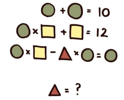
Example: Z3

• Z3 is an SMT solver developed by Microsoft Resarch.
• The tutorial [2] gives you a detailed introduction.
• Here is an example with Z3 from [1] - solving the puzzle
  below:

Example: Z3 (cont’d)

• If we use Z3’s Python interface, all we have to write is:
  #!/ usr/bin/ python
  from z3 import *
  circle, square, triangle
      = Ints(’ circle square triangle ’)
  s = Solver()
  s.add(circle + circle == 10)
  s.add(circle * square + square == 12)
  s.add(circle * square - triangle * circle == circle)
  print s.check()
  print s.model()

Example: Z3 (cont’d)

• Output:
  sat
  [triangle = 1, square = 2, circle = 5]

Satisfiability Modulo Theories

• SMT solvers take into account background theories, such as
  the theory of real numbers, the theory of integers, and the
  theories of various data structures such as lists, arrays, bit
  vectors, etc.
• Early approaches (“eager approaches”) translated SMT
  instances into Boolean SAT instances to solve them.
• More recent approaches (“lazy approaches”) integrate the
  Boolean reasoning of a DPLL-style search with theory-specific
  solvers (T-solvers) that handle conjunctions of predicates from
  a given theory.

Z3 Architecture

Another Example with Z3

• Here is another Z3 example from [1].
• Suppose we have an equation system:

• You can probably imagine how this would look in the Python
  interface.
• Python (and other high-level programming languages like C#)
  interfaces are highly popular, because they are practical.
• But actually there is a standard, LISP-like language for
  SMT-solvers called SMT-LIB.

Another Example with Z3

• The equation system in SMT-LIB:
  (declare-const x Real)
  (declare-const y Real)
  (declare-const z Real)
  (assert (=( -(+(* 3 x) (* 2 y)) z) 1))
  (assert (=(+( -(* 2 x) (* 2 y)) (* 4 z)) -2))
  (assert (=( -(+ (- 0 x) (* 0.5 y)) z) 0))
  (check-sat)
  (get-model)

Another Example with Z3

• Z3 will return:
  % z3 -smt2 example   .smt
  sat
  (model
    (define-fun z ()   Real
      (- 2.0))
    (define-fun y ()   Real
      (- 2.0))
    (define-fun x ()   Real
      1.0)
  )

List of SMT Solvers

• Alt-Ergo, https://alt-ergo.ocamlpro.com/
• Boolector, http://fmv.jku.at/boolector/
• CVC3/CVC4, http://cvc4.stanford.edu/
• dReal, http://dreal.cs.cmu.edu,
 https://github.com/dreal
• MathSAT, http://mathsat.fbk.eu/
• MK85, https://github.com/DennisYurichev/MK85
• STP, https://github.com/stp/stp
• toysolver, https://github.com/msakai/toysolver
• veriT, http://www.verit-solver.org/
• Yices, http://yices.csl.sri.com/
• Z3, https://github.com/Z3Prover/z3

SMT in Software Engineering (from [3])

• Dynamic symbolic execution (collect explored program paths
  as formulas, use solvers to identify new test inputs that can
  steer execution into new branches)
• Program model checking (automatically check for freedom
  from selected categories of errors, explore all possible
  executions)
• Static program analysis (check feasibility of program paths,
  not requiring execution)
• Program verification (assign logical assertions to programs)
• Modeling (high-level software modeling, making use of
  domain theories)

Example: Program model checking

             Is it possible to exit the loop
             without having a lock?

Example: Program model checking
Use SMT solver for constructing
finite-state abstractions.
  • Boolean variable b to encode
    the relation count ==
    old count
  • if (b) b = false; else b
    = *; to encode the abstraction
    of count = count+1
  • relation computed by an SMT
    solver by proving
    count==old count →
    count+1!=old count
  • * to represent a Boolean
    expression that
    nondeterministically evaluates
    to true or false

Example: Program model checking

               • abstract program with only
                 Boolean variables: finite
                 number of states
               • a finite-state model checker
                 can now be used on the
                 program and will establish that
                 b is always true when control
                 reaches this statement
               • i.e. calls to lock() in the
                 original program are balanced
                 with calls to unlock()

Example: Program verification

• Program verification
  applications often use theories
  not already supported by
  existing specialized solvers.
• But supported indirectly using
  axiomatizations with
  quantifiers.
• For example: Theory describing
  that objects in OO type
  systems are related using a
  single inheritance scheme
  (sub).

In This Course

• Propositional theorem proving (last Monday),
  Chapter 2 of the lecture notes
• First-order theorem proving (last Wednesday),
  Chapter 3 of the lecture notes
• Clause sets and resolution (Monday),
  Chapters 4 and 5 of the lecture notes
• Satisfiability checkers, SAT/SMT (today),
  Chapter 6 of the lecture notes, additional material