AWE-GEN-2d Nadav Peleg, Simone Fatichi, Athanasios Paschalis, Peter Molnar, Paolo Burlando
←
→
Page content transcription
If your browser does not render page correctly, please read the page content below

AWE-GEN-2d
Nadav Peleg, Simone Fatichi, Athanasios Paschalis,
 Peter Molnar, Paolo Burlando

 SWGEN-Hydro
 Berlin, 2017

Outline
1. Motivation and general overview
2. AWE-GEN-2d structure
3. Short demo
4. Advantages and weaknesses – from model validation
5. Applications
6. Next steps
Motivation
The potential to narrow uncertainty in projections of regional precipitation change (Clim Dyn)

 Local scale Local scale

 Hawkins and Sutton (2011)

Motivation
Uncertainty partition challenges the predictability of vital details of climate change (Earth’s Future)

 Local scale

 Natural climate variability is important also at small- local-scales!

 Fatichi et al. (2016)

Motivation
Some impact studies require high-resolution climate data, e.g. for estimating
streamflow in Alpine catchments (snow melt, glacier retreat, soil properties).

Gap – to the best of our knowledge, no sub-daily sub-kilometer stochastic weather
generator exists.

Solution – Yes, another weather generator!
AWE-GEN-2d in a nutshell
• AWE-GEN-2d (Advanced WEather GENerator for 2-Dimensional grid) follows the
 philosophy of combining physical and stochastic approaches to generate gridded
 climate variables in a high spatial and temporal resolution.

AWE-GEN-2d in a nutshell
• AWE-GEN-2d (Advanced WEather GENerator for 2-Dimensional grid) follows the
 philosophy of combining physical and stochastic approaches to generate gridded
 climate variables in a high spatial and temporal resolution.
• It is relatively fast and parsimonious in terms of computational demand.
• It allows generating many stochastic realizations of present and future climates.

Ancestors

 AWE-GEN-2d model
 Peleg et al. (2017)

HiReS-WG model
Peleg and Morin (2014)
Climate variables • Sub-daily temporal resolution. • Similar output as of AWE-GEN model, but meteorological variables are spatially distributed: Precipitation Cloud cover Temperature Radiation (incoming longwave, incoming shortwave, diffusive) Relative humidity Vapor pressure Atmospheric pressure Wind speed
Model structure
• Composed of eight modules.
• There is dependency between most, but not all,
 meteorological variables.

 LWR
Storm mean areal statistics

 Paschalis et al. (2013)
Storm mean areal statistics
• WAR-IMF-CAR process
• Matérn cross-covariance function for tri-variate random time-series (using the
 Parsimonious Multivariate Matérn model, Gneiting et al., 2010).

 Paschalis et al. (2013)
Precipitation
• The simulated WAR and IMF time series for each storm are transformed into the space-
 time evolution of the precipitation fields using latent Gaussian fields (simulated using 2-D
 FFT method).

 Nerini et al. (2017)
Precipitation
• The fields takes into account the exponential decay of the spatial autocorrelation (spectral
 density analysis) and the ARMA process (temporal correlation).

 Peleg et al. (2017c)
Precipitation and advection
• Due to the symmetries of the fast Fourier transform the generated fields can be folded.

 Paschalis et al. (2013)
Interitmtent precipitation fields
• Lognormal distribution (Paschalis et al., 2013):
 , , = −1 ( , , ) , , It looks like rainfall!
 ( )
 = But… precipitation are
 ( ) 2 + 1
 = 2 + 1
 homogenous at space

• Weibull distribution (Skinner et al., 2017):
 , , = −1 ( , , ) , ,
 2
 Γ 1+
 ( )2 2 + 1 =
 1 2
 Γ 1+

 ( )
 =
 1
 Γ 1 + ( )

 Paschalis et al. (2013)
Precipitation occurrence filter
U[G(x,y)] R(x,y)

 Precipitation
UWAR=0.5[G(x,y)] UWAR=0.5[G*(x,y)]
 occurrence
 filter
Precipitation intensity filter
Quantile [-]

 Direct link to GCM/RCM

 Extreme rainfall intensity are
 overestimated (at sub-hourly scales)

 Daily rain [mm]
Cloud cover
• During the intra-storm period, the cloudiness and rainfall fields are cross-correlated and
 cloud cover has always an equal or larger extent than the precipitation field.
• During an inter-storm period, the existence of a ‘‘fair weather’’ region is assumed,
 meaning that the cloudiness decreases as a function of the time passed since the end of
 the previous storm and increases toward the beginning of the next storm, using a two
 term exponential function.
• The stochastic component of the cloud cover series during an inter-storm period is
 simulated through an ARMA model.
Near-surface air temperature
• Air temperature is generated with an hourly time step first for a given reference level and
 then spatially extrapolated to all grid cells using a stochastic lapse rate.
• The deterministic temperature component is assumed to be directly related to the
 incoming longwave radiation and to the hourly position of the Sun and site geographic
 location.
• The stochastic temperature component is estimated through an autoregressive model
 AR(1).
• The air temperature at a given reference level can be generated with or without
 considering the shading effect of the terrain. The shadow effect is calculated as a binary
 coefficient: the sloping surface is shadowed by neighboring terrain (==0) when the
 horizon angle is lower than the zenith angle for a given solar azimuth.
Near-surface wind speed
• Near-surface wind speed is computed from the geostrophic wind speed.
• The near-surface wind speed is calculated using the geostrophic drag law (mass
 conservation component is not implemented), which requires a simplified computation of
 the Monin-Obukhov length, the friction velocity per grid cell, and the PBL height.
• The atmospheric stability is determined through the Pasquill stability classes (from
 extreme unstable to very stable atmospheric conditions), which is determined based on
 the shortwave incoming solar radiation and the cloud cover.
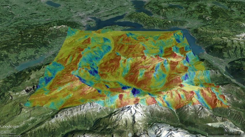
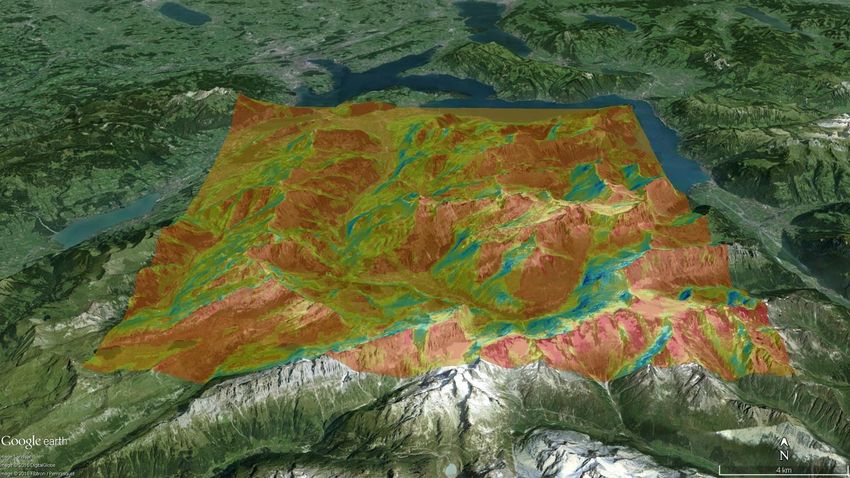
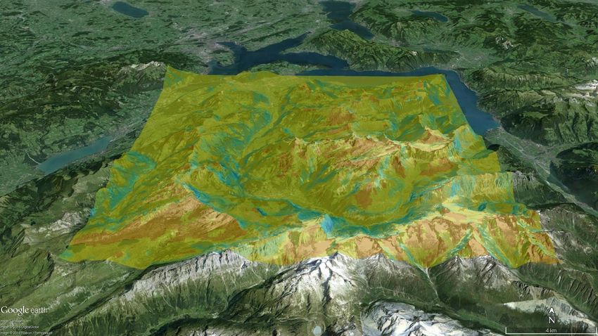
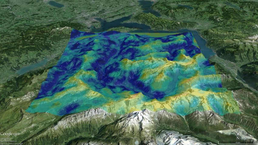
Case study: Engelberger catchment
 Domain size: 25 km by 25 km
 Elevation: 404 m to 3238 m
 Luzern
 Pilatus

 Altdorf

 Engelberg

 Titlis
Rainfall Fields
Spatial resolution of 2 km by 2 km
Temporal resolution of 5 min
 * Interpolated to a 100 m by 100 m grid for this example
High intensity cell
 evolving in time
 and space

 00:20 pm
 Advection

 Rainfall intensity [mm h-1]
 5 m s-1
High intensity cell
 evolving in time
 and space

 00:25 pm

 Rainfall intensity [mm h-1]
High intensity cell
 evolving in time
 and space

 00:30 pm

 Rainfall intensity [mm h-1]
High intensity cell
 evolving in time
 and space

 00:35 pm

 Rainfall intensity [mm h-1]
High intensity cell
 evolving in time
 and space

 00:40 pm

 Rainfall intensity [mm h-1]
Temperature Fields
Spatial resolution of 100 m by 100 m
Temporal resolution of 1 hour
06:00 am

 Temperature [°C]
 Jun, 17th

Engelberg

 Titlis
07:00 am

 Temperature [°C]
 Jun, 17th

Engelberg

 Titlis
08:00 am

Temperature [°C]
 Jun, 17th
09:00 am

Temperature [°C]
 Jun, 17th
10:00 am

Temperature [°C]
 Jun, 17th
11:00 am

Temperature [°C]
 Jun, 17th
12:00 pm
Mean cloud cover for June, 17: 0.37
Mean cloud cover for June, 18: 0.13

 Temperature [°C]
 Jun, 17th
12:00 pm
Mean cloud cover for June, 17: 0.37
Mean cloud cover for June, 18: 0.13

 Temperature [°C]
 Jun, 18th
01:00 pm

Temperature [°C]
 Jun, 18th
02:00 pm

Temperature [°C]
 Jun, 18th
03:00 pm

Temperature [°C]
 Jun, 18th
04:00 pm

Temperature [°C]
 Jun, 18th
05:00 pm

Temperature [°C]
 Jun, 18th
06:00 pm

Temperature [°C]
 Jun, 18th
Shortwave Incoming Radiation
Fields
Spatial resolution of 100 m by 100 m
Temporal resolution of 1 hour
06:00 am

 Incoming radiation [W m-2]
 Jun, 17th

Engelberg

 Titlis
Incoming radiation [W m-2]
Jun, 17th
 07:00 am
Incoming radiation [W m-2]
Jun, 17th
 08:00 am
Incoming radiation [W m-2]
Jun, 17th
 09:00 am
Incoming radiation [W m-2]
Jun, 17th
 10:00 am
Incoming radiation [W m-2]
Jun, 17th
 11:00 am
Incoming radiation [W m-2]
Jun, 17th
 12:00 pm
Incoming radiation [W m-2]
Jun, 17th
 01:00 pm
Incoming radiation [W m-2]
Jun, 17th
 02:00 pm
Incoming radiation [W m-2]
Jun, 17th
 03:00 pm
Incoming radiation [W m-2]
Jun, 17th
 04:00 pm
Incoming radiation [W m-2]
Jun, 17th
 05:00 pm
Incoming radiation [W m-2]
Jun, 17th
 06:00 pm
Near-Surface Wind Speed (2-m)
Spatial resolution of 100 m by 100 m
Temporal resolution of 1 hour
Wind speed [m s-1]
Inputs
Precipitation

 Advantages and weaknesses

• Spatial patterns are well represented
• Rainfall at daily scale is well reproduced

• Model overestimate extreme rainfall
 intensity at sub-daily resolution

 • Obs.: 30 years of data
 • Sim.: 50 realizations, each of 30 years
Temperature

 Advantages and weaknesses

• Hourly temperatures and dynamics are well represented

• Thermal inversion is simulated but is not validated
Shortwave radiation

Advantages and weaknesses
Vapor pressure

Advantages and weaknesses

 • In general good
 representation

 • Hourly dynamics are not
 fully capture
Wind speed

Advantages and weaknesses

 • Wind speed are not well
 represented at higher
 elevations
Applications
High spatio-temporal resolution climate scenarios for snowmelt modelling in small alpine
catchments
Schirmer et al. (ongoing)
Applications
Melt and surface sublimation across a glacier in a dry environment: distributed energy-
balance modelling of Juncal Norte Glacier, Chile
Ayala et al. (2017)
Applications
• Spatial variability of extreme rainfall at radar subpixel scale (Peleg et al., 2016)
• Partitioning the impacts of spatial and climatological rainfall variability in urban drainage modeling (Peleg et al., 2017)
• Rainfall-discharge-sediment yield uncertainty cascade in a second generation landscape evolution models (Skinner et al.)
• Simulating the effect of check dams on landscape evolution at centennial time scales (Ramirez et al.)
Future development
 • Re-parameterization AWE-GEN-2d for future climate
 • Diurnal cycle for precipitation (asymmetry?)
 • Coupling precipitation with temperature (extremes) Future

 • Replacing/improving wind estimates
2021-2030 2081-2090
 Present
Thank you for your attention!

Dr. Nadav Peleg
Research Associate
Hydrology and Water Resources Management
Institute of Environmental Engineering (IfU)
ETH Zurich

HIL D21.1
Stefano-Franscini-Platz 5
8093 Zurich, Switzerland
Office +41 44 633 27 17

nadav.peleg@sccer-soe.ethz.ch

AWE-GEN-2d paper:
Peleg, N., Fatichi, S., Paschalis, A., Molnar, P., and Burlando, P. (2017): An advanced stochastic weather generator for simulating 2-D
high resolution climate variables. Journal of Advances in Modeling Earth Systems, 9, p. 1595-1627.
You can also read