BAV MAGAZINE SPECTROSCOPY - OF THE GERMAN ORGANIZATION & WORKING GROUP VARIABLE STARS BAV
←
→
Page content transcription
If your browser does not render page correctly, please read the page content below
BAV Magazine
      SPEcTRoscopy

of the German Organization
             &
      working group
     Variable stars BAV
                    Editor
      Bundesdeutsche Arbeitsgemeinschaft
       Für Veränderliche Sterne e.V. (BAV)
               Munsterdamm 90
                 12169 Berlin

       Issue NO. 09   06/2021 ISSN 2566-5103
BAV Magazine
                                 SPEcTRoscopy

                                          EDITORIAL

     From the stars we basically receive only their electromagnetic radiation of different
wavelengths, and we “see” essentially only the surface of the radiating bodies. By evaluating the
light, we obtain information about:

   •   the direction of the radiation (positions and movement of the stars)
   •   the quantity of the radiation (brightness)
   •   the quality of the radiation (color, spectrum, polarization)

   For amateurs, only the narrow band of visible light is easily accessible. In this spectral region,
however, both the brightness (photometry) and the spectra of the objects can be examined.
Today's amateur astronomy, with its instrumental and computer-assisted equipment, enjoys
observation possibilities that were reserved exclusively for professional astronomers until a few
years ago.

   Thanks to the development of CCD technology, the types of observational perspectives have
become much more varied. For example, in the area of variable star observation, there are many
new possibilities in addition to already existing approaches.

   Professional variable star research employs techniques and observation methods to study the
physics and atmospheres of the stars in a holistic manner, considering all aspects and
occurrences. Thus, this means that the collected radiation must be understood as a complex
storage medium of the physical processes on and in the observed star.

   This is appropriate for the intensity of the light, as well as for its spectral composition. The
linking of brightness measurements and spectroscopy, a matter of course in professional
astronomy, reflects this connection.

   Along with brightness changes that occur in variable stars (which can occur quite frequently)
variable changes in the state of the stars also can take place and often are revealed in the
corresponding spectrum.

Ernst Pollmann

                               BAV MAGAZINE SPECTROSCOPY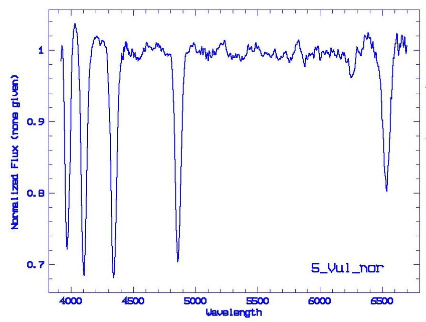
BAV Magazine
                            SPEcTRoscopy

Imprint
The BAV MAGAZINE SPECTROSCOPY appears half-yearly from June 2017. Responsibilty
for publication: German Working Group for Variable Stars e.V. (BAV), Munsterdamm 90,
12169 Berlin

Editorial
Ernst Pollmann, 51375 Leverkusen, Emil-Nolde-Straße 12, ernst-pollmann@t-online.de
Lienhard Pagel, 18311, Klockenhagen Mecklenburger Str. 87, lienhard.pagel@t-online.de
Roland Bücke, 21035 Hamburg, Anna von Gierke Ring 147, rb@buecke.de
The authors are responsible for their contributions.
Cover picture: wikipedia.org 2020/17/May

Content                                                                        Page

E. Pollmann: Editorial

P. Drake: Determination of the physical properties of the
          gamma Cassiopeia stellar system (Part II)                              1

K. Kiosseoglou: Harvard-Spekralklassifikation von Sternen und
                Einordnung im HRD                                               12

M. Sblewski: Photometry and Spectroscopy of Collinder 399                       31

R. Bücke: Polaris - Radialgeschwindigkeitsmessungen
          von 2005 bis 2020                                                     43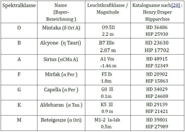
BAV Magazine
                                  SPEcTRoscopy

                            Determination of the physical properties
                        of the gamma Cassiopeia stellar system (Part II)
                            Pablo Drake (IES Rosa Chacel, Madrid, Spain)
                                 Prof. Dr. Felipe Perucho Gonzales

                    Abstract
                    In this monograph, we propose to determine the physical properties of the
                    binary star system Gamma Cassiopeia (γ Cas) by answering the questions:
                    1) What are the orbital characteristics of the binary system γ Cas, such as the
                    masses of both primary and secondary stars?
                    2) The shape and material composition of the primary star?
                    3) The maximum radial velocity of the secondary star, orbital period and semi
                    major axis (a) of its orbit? For this purpose, we have analyzed approximately
                    350 spectra. From each one of them we have obtained the value of the
                    Doppler shift, the rotational radial velocities of the primary star and the
orbital radial velocities of the secondary star. We conclude that the primary star shows a gas disk
composed of hydrogen and, closer to the center of the star, helium, with the mass of hydrogen
increasing. In addition, from the secondary star we have determined the values of its maximum
radial velocity, K = (4.29 ± 0.06) km s-1, of its orbital period, P = (203.46 ± 0.04) days, of its
mass, M2 = 0.9 solar masses, and of the semi major axis of it’s orbit, a = 400 solar radii.

   In relation to the quality and uncertainty of the spectra, both bases of data use professional and
amateur measurements however, the resolution of the spectrographs used can vary
significantly.The equivalent width Ew of each spectrum was found, by reducing the 350 Hα
spectra in VSpec. This application calculates the value of the equivalent width by selecting two
points on both sides of the emission line: from 6525 to 6610 Å, as shown in Fig. 12.

                                                                Fig. 12:
                                                                VSpec analysis of the γCas
                                                                20091225-spectrum (BeSS
                                                                database). Determination of
                                                    6610 A
                    6525 A

                                                                the EW within the wavelength
                                                                section 6525 to 6610 Å
                                                                (EW=-33.02 Å)

                               BAV MAGAZINE SPECTROSCOPY                                                1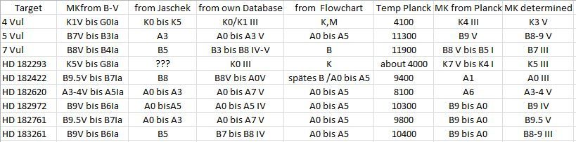
BAV Magazine
                           SPEcTRoscopy

                                                            Physical properties of gamma Cas

                                                                           Hß

                                                                           Hα

                                                                           He6678

Fig. 13: Temporal successions of the emission lines of Hβ, Hα and He 6678, from top to
       bottom. The x-axis represents wavelength, the y-axis the relative intensity.

                         BAV MAGAZINE SPECTROSCOPY                                             2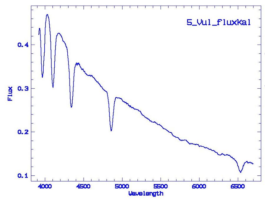
BAV Magazine
                                SPEcTRoscopy

                                                                  Physical properties of gamma Cas

   To develop the analysis, we begin by defining the variables to be studied and their notation.
As stated above, for the different reductions the independent variable is always time t (moment
of capture of the spectra) measured on Julian Date (JD). The dependent variable in the first
reduction is the rotational radial velocity νRr, measured in km s-1. In the second reduction, the
dependent variable will be the radial velocity vr of the secondary star, measured in km s-1.
Finally, in the third reduction, the dependent variable will be the equivalent width, Ew,
measured in Å.

   During the observation, we take as controlled variables both the radial heliocentric speed
(calculated by taking into account the time at which the spectrum is obtained and the
geographical location from which the observation was made) and the resolution of the spectra
(obtained from the databases).

   Data analysis
   Rotational radial velocity and structure of the main star.

   From the analysis of different spectral sequences of the spectral lines Hβ, Hα and He 6678 in
Fig. 13, we can observe a common pattern. It can be seen over time, that the graphs always
present two maxima around the theoretical emission line.

                                 Fig. 14: He 6678 emission line.
              The red line indicates the laboratory wavelength of the emission line.

   In Fig. 14 we can observe how these graphs show both a displacement to the red and to the
blue (with respect to the laboratory line). It indicates that the emission is produced by the time
approaching and receding from the observer. From Kirchhoff’s second law, we know that there
must be a gaseous mass that approaches and moves away from us continuously, and that it
contains hydrogen and helium.

                              BAV MAGAZINE SPECTROSCOPY                                              3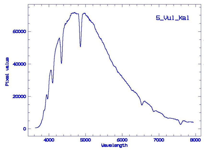
BAV Magazine
                                SPEcTRoscopy

                                                                   Physical properties of gamma Cas

   The best possible explanation for this (at present) is that the secondary star, due to its high
rotation speed has been deformed to create a gas disc around the main primary star. The radial
velocities of this rotational disc can be found by measuring the Doppler shifts of the maximum
and minimum emissions. We will analyze below those minimums for the case of the spectra of
He 6678 previously shown in Fig. 13.

                  Fig. 15: BeSS-spectra of He 6678 and corresponding lines,
     minimum wavelengths shifted to the blue, minimum wavelengths shifted to the red.
Uncertainties in wavelength values are obtained by reducing the spectra in VSpec. The value, Δλ
             = 0.0275 Å, can be expressed, to one significant figure, Δλ = 0.03 Å.

       Fig. 16: Table of heliocentric radial velocities showing maximum and minimum radial
 rotation velocity for the previous spectra, associated with each spectrum as different values of
                    rotational radial velocity for the wavelengths in Figure 15.

                              BAV MAGAZINE SPECTROSCOPY                                               4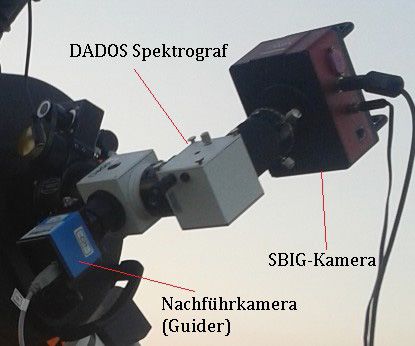
BAV Magazine
                                 SPEcTRoscopy

                                                                    Physical properties of gamma Cas

The values of Figure 16 were obtained from the formula

taking for λe the value of the emission line of He 6678 at 6678.1517 Å. For the spectrum γ
Cas_He 6678_20130706:

Regarding the absolute uncertainty, from the formula

we can deduce that, as c and λ are considered constants:
And in this case:

Next, we will make the correction of the rotational radial velocities with the heliocentric radial
velocity data for Figure 16, by adding them thus (´νRr neg = νRr neg + VRH).

 Fig. 17: Table with the values of the heliocentric radial velocity and the corrected values of the
                                     rotational radial velocity.

   By calculating the average value of the data obtained in Fig. 17, we obtain the average radial
velocity values in Fig. 18.

                              BAV MAGAZINE SPECTROSCOPY                                                5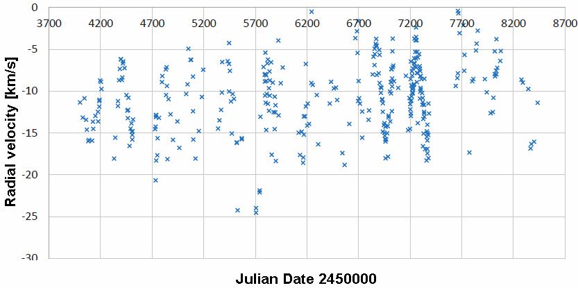
BAV Magazine
                                SPEcTRoscopy

                                                                   Physical properties of gamma Cas

     Fig. 18: Table with average rotational radial speeds and their respective uncertainties.

The uncertainty of the average was calculated using the expression: ∆ν = (maximum value -
minimum value)/2. For HeI 6678 with its positive values:

          ∆νRr = maximum value - minimum value)/2 = (264 –197)/2 = 33.5 = 30

Radial velocity of the secondary star: Orbital characteristics.

   To calculate the parameters of the orbit for the secondary star it is necessary to find the
temporal evolution of its radial velocity. With the temporal sample range (July to December
2015), the analysis of radial velocities over time gave the following result in Fig. 19-

                           Fig. 19: Radial velocity versus Julian date

                              BAV MAGAZINE SPECTROSCOPY                                               6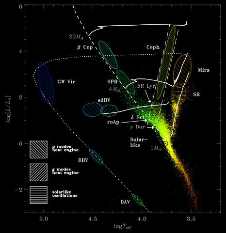
BAV Magazine
                                 SPEcTRoscopy

                                                                   Physical properties of gamma Cas

   The uncertainties for the ordinate were calculated, taking into account that the uncertainty for
each spectrometer is different, with the expression Δνr = (c Δλ0) / λe for each value. For the
abscissa, uncertainties are Δt ± 0.001 jd, so they are not significant. We can observe (especially
in Figure 20) a periodic trend in the graph that corresponds to predictions.

  Next, we calculate a sinusoidal approximation of the data values with the online program
ZunZunSite3. The solution is expressed in the form:

      Fig. 20: Radial velocity versus Julian Date; sinusoidal adjustment with ZunZunSite3.

The adjustment function has the following parameters:

                                       A   = -4.72 ± 0.06
                                       c   = 200 ± 500
                                       w   = 99 ± 1
                                       d   = -10.26 ± 0.03

   Since the program does not allow introducing of error bars, it was decided to add and subtract
respectively the absolute uncertainties to the data points and calculate two other approximations,
to see if the difference with respect to the original parameters was greater than the uncertainty
presented by the program. The results are as follows:

                              BAV MAGAZINE SPECTROSCOPY                                               7
BAV Magazine
SPEcTRoscopy
Physical properties of gamma Cas
AM = 4.82 ± 0.2 Am = -3.7 ± 0.2
cM = -100 ± 1700 cm = 300 ± 8600
wM = 101 ± 3 wm = 103 ± 4
dM = -7.62 ± 0.09 dm = - 13.3 ± 0.02
As we can see, the difference of the original parameters with respect to these maximum and
minimum approximations is greater than their uncertainties, so we can rewrite the parameters
with the new uncertainties:
A = -4 ± 1
c = 200 ± 500
w = 99 ± 4
d = -10 ± 3
From these parameters, we can deduce two orbital elements for this sample group, namely
the maximum K of the radial velocity, and the period P of the orbit. In particular, K will be
directly equal to parameter A, since it is equivalent to the amplitude of the function. As for the
period P, its calculation requires a series of mathematical transformations
Km = A = (-4 ± 1) km s-1
Pm = 2w = 2(99 ± 4) = (198 ± 8) days
Next, combining this sample with the total range.set of data studied.
Fig 21: Radial velocity versus Julian date; General range.
BAV MAGAZINE SPECTROSCOPY 8BAV Magazine
SPEcTRoscopy
Physical properties of gamma Cas
Fig. 22: Radial velocity versus Julian date; sinusoidal adjustment with ZunZunSite3.
The following parameters are obtained:
A = 4.29 ± 0.06
c = -500 ± 100
w = 101.73 ± 0.02
d = -10.98 ± 0.02
And therefore,
Kg = A = (4.29 ± 0.06) km s; Pg = 2w = 2(101.73 ± 0.02) = 203.46 d (± 0.04)
To corroborate the accuracy of the results, we include a phase diagram. To do this, we define
a time t0 such that the orbital phase at t0 is equal to 0. We establish that for t + nP (for n = ℕ), the
phase is 0 such that all periods accumulate in the same phase.
Fig. 23: Radial velocity versus Phase.
BAV MAGAZINE SPECTROSCOPY 9BAV Magazine
SPEcTRoscopy
Physical properties of gamma Cas
We observe in Fig. 23 that the sample values of the radial velocity along the phase are
distributed in a similar way to the general values. As we can see in Figure 24, the range of
uncertainties is unequal, with much larger error bars for the lower values of time. This causes the
previously used method to find uncertainties, to yield inconclusive results, by making a complete
adjustment of the data impossible.
Fig. 24: Radial Speed versus Julian date; Includes uncertainties.
Equivalent width of the Hα line
For the spectra of the Hα emission line, the equivalent width Ew has been studied in addition
to the radial velocity, resulting in Fig. 25.
Fig. 25: Equivalent versus Julian date; Linear approximation
BAV MAGAZINE SPECTROSCOPY 10BAV Magazine
SPEcTRoscopy
Physical properties of gamma Cas
For this data we have calculated an uncertainty of ΔEw = 0.5 Å. It can be deduced that they
seem to follow a linear distribution that responds to the adjustment Ew = -0.0033t – 12.046. On
the other hand, we conclude that the equivalent width of the Hα line decreases gradually
according to the expression Ew = -0.0033t – 12.046.
Conclusions
In this investigation, the following results are found in relation to the characteristics of the
binary system γ Cas. First, we have found that the main star is surrounded by a disk of hydrogen
and helium gas. These elements rotate with radial velocities as shown in Fig. 18, in which it can
be seen that the rotational radial velocity of helium is greater than that of hydrogen. We know
that the bodies closest to a central mass rotate faster than the distant ones. This allows us to
deduce that, within the gas disk, helium is closer to the stellar nucleus than hydrogen, and Hα
emission will come, consequently, from the outer parts of the disk. This has been impressively
described with the Fig. 28 below, developed by Stee et al. 1998.
Fig. 26: Spectral distribution of the γ Cas disk.
(from Stee et al: Astron. Astrophys. 332, 268-272, 1998)
Thanks to Jack Martin (UK) for translating the article.
Part I of this work have been published in this magazine issue No. 08, 12/2020
BAV MAGAZINE SPECTROSCOPY 11BAV Magazine
SPEcTRoscopy
Harvard-Spektralklassifikation von Sternen und
Einordnung im Hertzsprung-Russell Diagramm (Teil II)
Konstantinos Kiosseoglou
Praktischer Teil
Die Spektren wurden in der Schulersternwarte des Carl-Fuhlrott-
Gymnasiums aufgenommen. Die Sternwarte besteht seit 2009 und
ermöglicht Schülern und Besuchern den den Zugang zur Astronomie,
angefangen mit einem ersten Einblick in diese Wissenschaft bis hin zu
umfangreichen Projektarbeiten. Die Arbeitsprojekte können sowohl am
Hauptteleskop im zentralen Astrolabor, als auch an den sechs
Arbeitsstationen, die sich benachbart auf dem Schuldach befinden, umgesetzt
werden. Die Stationen werden mit einem Materialwagen aus dem Astrolabor angefahren und
enthalten bis auf das C11-Teleskop unterschiedlichste Ausrüstung wie Filter, Kameras und
Okulare, die bei jeder Messung aufgebaut und in Betrieb genommen werden müssen.
Aufbau, Messung
Vor der Messung musste die gesamte Messvorrichtung bestehend aus
Montierung: Astro-Physics 900GTO
Teleskop: Celestron 11‘‘(C11) EdgeHD
DADOS Spaltspektrograf mit 200 L/mm
CCD-Kamera: SBIG STF-8300M
Notebook mit der Software Maxim DL
in Betrieb genommen werden. Die Kernbestandteile der Ausrüstung sind Teleskop,
Spektrograph und Kamera. Das C11 ist ein Spiegelteleskop mit einer Brennweite von 2800mm
und erzeugt ein „auf dem Kopf stehendes Bild eines Objekts im Brennpunkt der Zwei-Spiegel-
Optik" [3]. Der Hauptspiegel (HS) hat einen Durchmesser von 28 cm (=11Zoll) und wird
mittels Justierschrauben zum fokussieren des Bildes gesteuert.
Abb. 17: Strahlengang des Celestron 11‘‘ (C11) EdgeHD‐Teleskop
BAV MAGAZINE SPECTROSCOPY 12BAV Magazine
SPEcTRoscopy
Harvard-Spektralklassifikation
Am Teleskop wurde der DADOS-Spaltspektrograph mit dem am geringsten auflösenden
Gitter mit 200 L/mm verwendet, damit der gesamte Spektralbereich der Spektren vollständig
auf den Kamerasensor abgebildet werden kann.
Abb.18: C11 mit DADOS Spektrograf und SBIG CCD Kamera
Das Teleskop muss vor der Spektrenaufnahme an einem größeren Objekt (Planet oder Mond)
fokussiert werden. Anschließend wird, ausgehend von der ersten Ordnung des Spektrographen,
entweder mit einer Kalibrierlampe oder einem anderen diskreten Spektrum, der gewünschte
Bereich an der Justierschraube des Spektrographen eingestellt, sowie das erzeugte Spektrum mit
dem Okular der Kamera optimal fokussiert.
Mit Hilfe der Teleskopsteuerung wird anschließend das gewünschte Objekt angefahren bis es
im Sucher mittig zu sehen ist.
Das Zielobjekt wird danach visuell über den Slit-Viewer am DADOS-Spektrographen im Spalt
positioniert und während der Spektralaufnahme mit der Steuerung der Montierung so gut wie
möglich stabil gehalten. Die Belichtungszeit wurde der Helligkeit des Sterns angepasst. Sie liegen
typischerweise zwischen 10 und 100 Sekunden.
BAV MAGAZINE SPECTROSCOPY 13BAV Magazine
SPEcTRoscopy
Harvard-Spektralklassifikation
Abb.19: Collage der Größenrelationen am Spalt
Tabelle: Beobachtungsobjekte der Messreihe
Die ausgewählten Beobachtungsobjekte decken die Spektralklassen ab und sind in obiger Tablle
aufgelistet. Die Spetrenaufnahme wird direkt am Notebook an einem Histogramm auf die
Eignung zur weiteren Auswertung bewertet, ggf. gespeichert und anschließend an den Server
übertagen.
BAV MAGAZINE SPECTROSCOPY 14BAV Magazine
SPEcTRoscopy
Harvard-Spektralklassifikation
Exemplarische Auswertung
Der Ablauf der Datenverarbeitung soll mit Hilfe der nachfolgenden Screenshots detailiert
erläutert werden. Die Beschreibungen der jeweiligen Arbeitsschritte findet sich unter den
Abbildungen.
Abb. 20.: Begradigen und Ausschneiden der Aufnahme mit Fitswork
Die Begradigung der Rohspektren wird mit der Software Fitswork vorgenommen. Die
Spektren werden geladen und mittels der Befehlskette Bearbeiten>Bildgeometrie>Bild rotieren an
der Hilfslinie ausgerichtet (volles Bild). Anschließend wird per Hand ein Rahmen ausgeschnitten
und gespeichert. Dieser sollte jedoch nicht zu knapp gezogen werden, da in ihm, ober- und
unterhalb des Spektralstreifens für das Auge nicht sichtbare Bildinformationen enthalten sind.
Abb. 21.: Erzeugen eines Rohspektrums mit VSPEC
Mit der Software VSPEC wird nun zuerst das aktuelle Arbeitsverzeichnis, in dem sich die
Daten befinden, mit Options>Perferences ausgewählt und mit Button > display reference binning zone
ein Rahmen erzeugt und über dem Spektralstreifen platziert. Der Button referenc binning erzeugt
automatisch ein Spektrum, in dem Fremd- oder Streulichtanteile heraus gemittelt werden. Das
erzeugte Spektrum wird als Rohspektrum bezeichnet, da es die optischen Eigenschaften der
gesamten Messkette enthält und noch nicht wellenlängenkalibriert ist.
Abb.22: Erzeugen eines synthetischen Spektrums
BAV MAGAZINE SPECTROSCOPY 15BAV Magazine
SPEcTRoscopy
Harvard-Spektralklassifikation
Bei wiederholten Bearbeitungsschritten ist es ratsam, das aktuelle Rohspektrum mit
Menü>Edit>replace>intensity im aktuellen Arbeitsspeicher zu speichern. Mit Tools>Synthesis wird
ein synthetisches Spektrum erzeugt, welches zur Orientierung dient und das Messergebnis
veranschaulicht.
Hδ Hγ Hß Hα
Abb.23: Auffinden der relevanten Spektrakllinien mit Hilfe eines Referenzspektrums
Im Standartverfahren wird vor einer Messung bzw. Messreihe ein Spektrum einer
Kalibrierlampe aufgenommen, da die Sichtung und Zuordnung von Spektren bzw. der Linien
ohne einen definierten Bezugsrahmen ein hohes Maß an Erfahrung benötigt. Die durch
Erfahrung erlernte Mustererkennung wird über ein Referenzspektrum nachvollzogen. Das
markanteste Muster hier ist die Balmerserie des Wasserstoffs.
Abb. 24: Kalibrieren des Rohspektrums mit Linien der Wasserstoff-Balmerserie
Mit Button>calibration multiple lines werden nun die in der VSpec-Hilfstabelle (rechts in Abb.
24) angegebenen Wellenlängen eingegeben, was der standardmäßigen Energie-Kanal Eichung
und der experimentellen Physik entspricht. Mit der Maus werden die Bereiche mit Hilfe einer
Lupenfunktion genau eingegrenzt. Der RMS-Wert (RootMeanSquare) bezeichnet den
Kalibrationsfehler, der nach Möglichkeit deutlichBAV Magazine
SPEcTRoscopy
Harvard-Spektralklassifikation
Abb. 25: Division durch ein Referenzspektrum aus Datenbank
Nach der Speicherung des wellenlängenkalibrierten Spektrums wird ein Bezugsspektrum
gleicher Spektralklasse aus der VSpec-Datenbank mit Menü>Assistant>Instrumental response
>>Button> Pickels ausgewählt und mit Button>Division and Extraction das kalibrierte Rohspektrum
durch dieses Bezugsspektrum dividiert, um die Instrumentenfunktion zu bestimmen.
Abb. 26.: Glätten der Instrumentenfunktion mittels Spline-Filter
Die so ermittelte Instrumentenfunktion wird mit Menü>Operatios>spline Filter und einem
Schieberegister (Regler), welches die entsprechenden Polynomkoeffizienten beinhaltet, geglättet
und gespeichert.
BAV MAGAZINE SPECTROSCOPY 17BAV Magazine
SPEcTRoscopy
Harvard-Spektralklassifikation
Abb. 27: Erzeugung eines flusskalibrierten Spektrums durch Division
Das wellenlängenkalibrierte Spektrum (Abb. 27 oben) wird durch die Instrumentenfunktion
(Abb. 27 unten) mit Menü>Operations>Divide a Profile by a Profile dividiert, wodurch das sog.
flusskalibrierte Spektrum in Abb. 28 erzeugt wird. Mit der Zunahme der Arbeitsschritte
verdeutlicht sich hier die Wichtigkeit funktionaler Bezeichnungen bei der Dateispeicherung.
Abb.28: Divisionsergebnis normieren und zuschneiden des Spektrums
Danach wird der Wellenlängenbereich von 5000-5050 A (siehe Abb. 28) mit dem Button
Normalize auf den Intensitätswert 1 normiert und der relevante Spektralbereich für die
Auswertung ausgeschnitten und gespeichert.
BAV MAGAZINE SPECTROSCOPY 18BAV Magazine
SPEcTRoscopy
Harvard-Spektralklassifikation
Abb. 29: Finales normiertes Flussspektrum mit synthetischem Spektrum
Das fertig normierte und flusskalibrierte Spektrum mit den identifizierten Absorptionslinien
wird zugeschnitten und mit einem synthetischen eingefärbten Spektrum zur Veranschaulichung
bzw. zur Verdeutlichung ergänzt.
Arbeitsschritte zur Einordnung in das Harvard Schema
Im Folgenden werden die Arbeitsschritte zur Einordnung in die Harvard-Klassifikation
dargestellt. In der folgenden Arbeitsweise entsprechend des Programmablaufplans (Abb. 30)
wird ausgehend von der Balmerserie, die Verteilung und die Intensität verschiedener
Absorptionslinien gesucht und anhand verschiedener Kriterien eingeordnet.
Abb. 30: Programmablaufplan zur Klassierung von Spektren
BAV MAGAZINE SPECTROSCOPY 19BAV Magazine
SPEcTRoscopy
Harvard-Spektralklassifikation
Mit diesem groben Arbeitsformalismus ist es auch Amateuren möglich, die grobe Klassierung
von Sternspektren vorzunehmen. Da das Auflösungsvermögen des DADOS Spektrographen bei
13,5 Å liegt und eine Vermessung der Linien relativ große Fehler produziert, reicht es aus, die
Intensitätsverhältnisse visuell mit dem Auge abzuschätzen.
Klassifizierung der Spektren
Die Spektren werden im folgendem Kapitel einzeln diskutiert, indem der Ablaufplan für das
jeweilige Spektrum überprüft wird und eine Aussage zur Einordnung erfolgt. Bezugspunkt ist
einerseits der Plot des Spektrums, andererseits jedoch auch mit Blick auf die
Entstehungsgeschichte der Klassifikation und das mit dem verarbeiteten Spektrum erzeugte
synthetische Spektrum. Die synthetischen Spektren sind zudem Software bedingt nicht im selben
Maßstab abgebildet wie der Plot. Dargestellt sind jeweils ein Bild der entsprechenden
Rohaufnahme, ein ausgewerteter und beschrifteter Plot (Intensität versus Wellenlänge) sowie ein
mit der Software VSpec synthetisch erzeugtes Spektrum. Die jeweiligen Entscheidungswege sind
als Ausschnitte der Abb. 30 mit Pfeilen zur Veranschaulichung der Entscheidungswege in eine
Abbildungskopie neben dem Text eingefügt.
Abb. 31: Mintaka
Das erste Maß im Alltagsgebrauch wäre die maxi-
male Intensität der Verteilung (hier im UV Bereich).
Im Plot fällt zunächst die Balmerserie und ihre geringe
Intensität auf. Durch die nicht vorhandenen Ca-Linien
endet hier schon die Einordnung mit der Klassierung
der Spektralklasse B. Im sw-Spektrum fällt zudem ein
wichtiges Muster zwischen Hβ und HeI auf. Da
Mintaka nach Hipparchos und dem Henry Draper Ka-
talog mit O9.5 klassiert wird zeigt sich, dass die Klas-
sierung mit fließenden Grenzen arbeitet und nicht
technisch über Interpretationen zustande kommt.
BAV MAGAZINE SPECTROSCOPY 20BAV Magazine
SPEcTRoscopy
Harvard-Spektralklassifikation
Abb. 32: Alcyone
Im Vergleich zu Mintaka sind die Absorptionslinien im sw-Spektrum deutlich intensiver und
das Muster ist klar zu erkennen. In der linken Hälfte fehlen auch hier die Fraunhoferlinien und K
für Calcium, also Klasse B (vergl. Tab. 4 in Teil I, 12/2020, >B7e). Das Suffix 'e' bezeichnet die
Emissionslinie von Hα. Dieser Sonderfall tritt bei Sternen mit einer Akkretionsscheibe um den
Stern ein, in der die Emission von Hα durch Emission in der Akkretionsscheibe entstehen,
welche überwiegend aus Wasserstoff besteht. Im Plot sind noch die tellurischen Linien
(Absorptionen in der Erdatmosphäre) für Sauerstoff zu sehen, welche die Software bei Bedarf für
eine Optimierung der Darstellung automatisch entfernen bzw. herausrechnen kann. Im Plot fällt
zunächst die Balmerserie und ihre geringe Intensität auf. Durch die nicht vorhandenen Ca-Linien
endet hier schon die Einordnung mit der Klassierung der Spektralklasse B. Im sw-Spektrum fällt
zudem ein wichtiges Muster zwischen Hß und HeI auf. Da Mintaka nach Hipparchos und dem
Henry Draper Katalog mit O9.5 klassiert wird, zeigt sich, dass die Klassierung mit fließenden
Grenzen arbeitet.
BAV MAGAZINE SPECTROSCOPY 21BAV Magazine
SPEcTRoscopy
Harvard-Spektralklassifikation
Abb. 33: Sirius A
In diesem Fall wird bezüglich der vorhandenen Ca-K-Linie das Intensitätsverhältnis zwischen
Ca-K zu Hγ im Plan berücksichtigt und endet bei A-A5. In diesem Fall sehr passend. Die
Balmerserie ist hier sehr markant ausgeprägt. Aus den letzten drei Spektren wird auch qualitativ
deutlich, dass sich das Maximum der Intensitätsverteilung in Richtung höherer Wellenlängen
verschiebt.
BAV MAGAZINE SPECTROSCOPY 22BAV Magazine
SPEcTRoscopy
Harvard-Spektralklassifikation
Abb. 34: Mirfak
Im sw-Spektrum sind jetzt links domi-
nante Ca Linien zu erkennen und das Spekt-
rum sieht im Ganzen gröber strukturiert
aus. Das Grundmuster der Balmerserie Hα
bis Hγ ist noch zu erkennen. Es sind jedoch
mit bloßem Auge ohne Vergrößerung kaum
Aussagen möglich. Im Plot erkennt man
jetzt Eisen und einen Ansatz einen Natri-
umlinie.
Aus dem Plan ergibt sich folgender
Weg:
Klasse A6-F (siehe Bild rechts). Die
Klassifizierung in Henry-Draper Katalog
wird mit FV1b angegeben. Zusätzlich zu
den bekannten Linien tritt eine neue Linie
auf, die CH Molekülbande (G) mit Vibrati-
ons- und Rotationszuständen [1, S. 246],
welche als Orientierungsmarke bei Spekt-
ren mit Calciumlinien helfen kann.
BAV MAGAZINE SPECTROSCOPY 23BAV Magazine
SPEcTRoscopy
Harvard-Spektralklassifikation
Abb. 35: Capella
In diesem sw-Spektrum sind wieder die
starken Fraunhoferlinien des Calciums zu
sehen und die Feinstrukturierung des
Spektrums nimmt zu. Die Balmerserie ist
noch zu erkennen, fügt sich jedoch merkbar
in den Hintergrund ein und ist ab dieser
Klasse als Orientierungspunkt für Kalibrati-
onen nicht mehr geeignet.
Neue Metalllinien des Magnesiums er-
scheinen im Plot. Im Ablauf (rechts) ent-
scheidet sich die Einordnung nach der Inter-
pretation der Linienstärke. Es kann jedoch
ungefähr von gleicher Intensität ausgegan-
gen werden, was schlussendlich zur Klasse
G0-G4 führt.
BAV MAGAZINE SPECTROSCOPY 24BAV Magazine
SPEcTRoscopy
Harvard-Spektralklassifikation
Abb.: 36: Aldebaran
Im sw-Spektrum sind nun breite dunkle Bereiche, sogenannte Bandenstrukturen zu erkennen,
ein klarer Hinweis auf eine späte Spektralklasse, welche dem Titanoxid zugeordnet werden kann.
Die Vielzahl der Metallabsorptionen hat eine beinahe verrauschte Struktur.
Eine Zuordnung auf der Basis der optischen Eindrücke wird kaum mehr möglich, da die
verwendete Auflösung hier an ihre Grenzen kommt. Es kann z.B. nicht zwischen Mg (5168-
5183Å) oder TiO (5168Å) unterschieden werden.
In dem sw-Spektrum sind dennoch die Ca Linien, meiner Einschätzung nach die CaH Linie, zu
erkennen, so dass der vorgezeichnete Weg nachvollziehbar ist. Die Schwierigkeit der Deutungen
in den Spektralklassen K und M zeigt sich schon daran, dass beide in derselben Klassifizierung im
Plan stehen. Bei der Wellenlängenkalibration mit nur 4 Stützstellen konnte lediglich ein RMS
Wert von 2.39 erreicht werden.
BAV MAGAZINE SPECTROSCOPY 25BAV Magazine
SPEcTRoscopy
Harvard-Spektralklassifikation
Abb. 37: Beteigeuze
Das gleiche Bild ergibt sich bei Beteigeuze. Mit Hilfe von Beispielspektren in [5] wurden noch
die Linien für Magnesium und Eisen gefunden, rein optisch ergibt sich jedoch derselbe Weg wie
bei Aldebaran. Die Klassifizierung endet hier bei K oder M.
Die rechte Bandenstruktur kann sowohl tellurischer Wasserdampf als auch Sauerstoff sein. In
der Wellenlängenkalibration mit 6 Stützstellen konnte lediglich ein RMS Wert von 1,76 erreicht
werden, was zudem die Verlässlichkeit der Zuordnung schwierig macht.
In R. Walkers Buch [4] existiert noch eine andere Variante, welche für die Unterscheidung
der Klassen K und M über die Linienintensitäten G-Band (4300- 4310Å) bzw. TiO (5168Å)
entscheidet. Dieser Weg führt jedoch in beiden Fallen zu keinem verlässlichen Ergebnis, da
entweder das G-Band oder die TiO-Bande nicht genau lokalisiert werden kann.
BAV MAGAZINE SPECTROSCOPY 26BAV Magazine
SPEcTRoscopy
Harvard-Spektralklassifikation
Einordnung der Ergebnisse
Abb.38: Einordnung der Spektralklassen in das HRD
Wie sich nunmehr zeigt, kann eine Zuordnung der Spektralklasse auf diesem Weg lediglich
eine erste Orientierung sein.
Der genaue Deutungszusammenhang über die realen Verhältnisse ist jedoch immer fraglich,
wie bereits bei der Spektralklassenzuordnung ersichtlich geworden ist. Beispielsweise sind die
Sterne Mintaka und Sirius Mehrfachsysteme, so dass in Bezug zur Eindeutigkeit und Belastbarkeit
der gemessenen Eigenschaften innerhalb eines komplexen Themengebietes nur mit modernsten
astronomischen Mitteln und Methoden eine genaue Zuordnung der relevanten Parameter
erfolgen kann, damit sie wissenschaftlichen Ansprüchen genügen können.
Das Herzsprung-Russell-Diagramm (Abb. 38) dient dabei als Orientierungs- und
Kontrollmethode. Die Unterscheidung der Spektralklassen hinsichtlich ihrer absoluten
Helligkeit findet aber erst über die Leuchtkraftklassen, die in der Tabelle (Seite 14) aufgelistet
sind, einen wirklichen Zusammenhang.
BAV MAGAZINE SPECTROSCOPY 27BAV Magazine
SPEcTRoscopy
Harvard-Spektralklassifikation
Problematisierung der Flusskalibrierung
Die Instrumentenfunktion ist durch eine Division mit einem Bezugsspektrum nach folgender
Beziehung entstanden:
In der Schar abweichender Instrumentenfunktionen in Abb. 39 ist jedoch erkennbar, dass
diese von weit mehr als nur von den verwendeten optischen Kernbauteilen der Messkette wie
Teleskop, Spektrograph und Kamera abhängt, obwohl sich eine gemeinsame Grundstruktur
zeigt. Zur Vergleichbarkeit der Funktionen wurden die Plots im abgebildeten
Wellenlängenbereich von 3500-7500 Å ausgeschnitten (Abb. 39).
Der Hauptgrund der Unterschiedlichkeit der Funktionen findet sich u. a. in den
atmosphärischen Bedingungen zur jeweiligen Aufnahmezeit am gegebenen Beobachtungsort. Da
schon unser blauer Tageshimmel eine Folge der Rayleigh-Streuung ist, gibt es zudem noch
weitere Bedingungen, die die Transmission elektromagnetischer Strahlung beeinflussen.
Aufsteigende warme Luft kann bspw. wie eine Linse wirken und chromatische Dispersion
verursachen
Die erste Erkenntnis bei spektroskopischen Aufnahmen ist demnach, dass eine präzise
Flusskalibration nur über eine sog. „Standardkerze“ bekannter Wellenlängenverteilung außerhalb
der Atmosphäre möglich ist. Deshalb wird in diesem Verfahren aus einer Datenbank ein mit
professionellen Mitteln gewonnenes normiertes Bezugsspektum gewählt, um sich dem 'wahren'
Flussbild des gemessenen Sterns 'anzunähern'.
Bei der Division des Rohspektrums durch die Instrumentenfunktion wird nach [2] der Fluss
des Bezugsspektrums in der Messung abgebildet. Leider gibt es mit den Mitteln der Sternwarte
des Carl-Fuhlrott-Gymnasiums keine alternative Lösung für dieses Problem.
Unter diesen Gesichtspunkten ist auch klar, warum eine Bestimmung der Effektivtemperatur
nach Planck keinen Sinn macht, da so lediglich die Temperatur des Bezugsterns dargestellt
würde. Die folgende Abb. 39 zeigt nun den Vergleich der im Rahmen dieser Arbeit ermittelten
Instrumentenfunktionen:
BAV MAGAZINE SPECTROSCOPY 28BAV Magazine
SPEcTRoscopy
Harvard-Spektralklassifikation
Abb.39: Instrumentenfunktionen aus allen hier vorgestellten Messungen
BAV MAGAZINE SPECTROSCOPY 29BAV Magazine
SPEcTRoscopy
Harvard-Spektralklassifikation
Fazit
Der eigenständige Projektkurs Astronomie am Carl-Fuhlrott-Gymnasium ist für Schüler der
Qualifikationsphase des Leistungskurses Physik der 11.Klasse (Q1) offen und eine der
Wahlmöglichkeiten zur Erbringung der benötigten Leistungsnachweise zur Zulassung der
Abschlussprüfung. Darüber hinaus können weiterführende Arbeiten als besondere Lernleistung
eingebracht werden, unter anderem zur Erarbeitung eines MINT-Zertifikates.
Den CFG-Projektkurs sehe ich als Exzellenzinitiative, dessen eigentlicher Zugewinn darin
besteht, dass Schüler sich mit praktischen Aspekten eines größeren Vorhabens insofern
auseinandersetzten, da sie über die Ergebnisse ihrer Arbeit im Zentrum des Prozesses stehen und
auf eine greifbare Erfahrung hinsichtlich Ergebnis und Performance stützen können. Vor allem
bietet das Fach Astronomie einen breiten interdisziplinaren Ansatz.
Im ganzen bin ich meinem Ziel, der Astronomie und ihren Methoden zur
Erkenntnisgewinnung ein Stück nähergekommen und sehe viele Möglichkeiten, das erworbene
Wissen im Regelunterricht einbringen zu können. Zuletzt möchte ich Herrn Koch für die gute
Betreuung und sein Engagement danken!
Referenzen
[1] Wilfried Kuhn (Hrsg.) Aulis Verlag, Hallbergmoos 2011
[2] Paul A. Tipler, Mosca, Gene, Oldenbourg Verlag, München 2010
[3] Koch Bernd: Teleskopkunde, Arbeitsmaterialien der Schulersternwarte des CFG
[4] Richard Walker: https://docplayer.org/10843605-Analyse-und-interpretation-
astronomischer Spektren.html
[5] Beispielspektren:http://www.sternwartehabichtswald.de/astromania/galerie/Spektren
Part I of this work have been published in this magazine issue No. 08, 12/2020
BAV MAGAZINE SPECTROSCOPY 30BAV Magazine
SPEcTRoscopy
Photometry and Spectroscopy of Collinder 399
Martin Sblewski, Strausberg, Germany, m8neptun@t-online.de
Abstract
Collinder 399 is a star cluster located in the constellation Vulpecula.
Wikipedia informs us that Collinder 399 was named by Per Collinder and has
been listed as an Open Star Cluster since 1931. Since the end of the 1980's,
professional astronomers have been investigating whether the stars in this
cluster are in a physical relationship or whether they are a random
accumulation of stars forming a so-called asterism. In this context, an
attempt was made to investigate this question with simple observational
devices available to amateurs. The observations, measurements, evaluations and results are
presented in the following.
Observation data and analysis pathway
Collinder 399 includes 10 stars with a brightness in V between 5-7mag., which on the one
hand are not too bright for photometry and on the other hand are still bright enough for
spectroscopy. Photometric images in filters B and V from November 2016 are available for the
analysis. In addition, there are spectroscopic images in low resolution taken in December 2016.
Fig. 1: Photo of Collinder 399
BAV MAGAZINE SPECTROSCOPY 31BAV Magazine
SPEcTRoscopy
Photometry and Spectroscopy of Collinder 399
The following questions were included in the investigation:
- Estimation of the spectral class on the basis of the colour index B-V
- Improvement of the spectral class determination by investigation of the spectral images
- Determination of the spectral class by measurement of equivalent widths and
comparison with references [1] on the normalized spectrum
- Determination of spectral class by measurement of equivalent widths and comparison
with data from my own database on normalized spectra
- Determination of the spectral class with flow chart [2] on the normalized spectrum
- Determination of the temperature with flux-calibrated spectra and Planck curve [8].
- Calculation of the distance with the distance modulus
- Comparison of the results with official values
Photometry, equipment, exposure data, processing
A setup consisting of a small apochromat with a diameter of 60mm and a reduced focal length
of 260mm coupled with a filter wheel and an Atik 383 L+ camera is used to record the
photometric data. In normal operation, variable stars are observed with this setup. The small
diameter of the optics allows exposure times for stars of the 4th-6th magnitude that are in the
range of seconds. This avoids saturation of the image pixels and allows the total exposure time of
60 seconds recommended by the AAVSO to be aimed for, to compensate for atmospheric
variations. The filter set consists of photometric filters that approximately correspond to the
Johnson UBVRI system. The camera's chip, a Kodak KAF-8300 in the B/W version, scores with
5.4µm pixels and a size of 3362 x 2504 pixels. This results in a field of view of approximately
4.5° x 3.4°, which is comfortably large to find sufficient comparison stars in addition to the
desired variable stars.
For the project, pictures were taken in the filters B, V and R, of which only B and V will be
used in the following. B was exposed for 10 x 10s and V for 20 x 1s; corresponding flat, dark and
bias exposures were made. The images were calibrated, aligned and stacked with the software
Maxim DL. The stacked images were then used in the V-Phot software, which is offered by the
AAVSO for image processing. Here, comparison and check stars can be loaded and the
brightness of the Collinder stars can be determined.
Absolute brightness, distance module
The absolute brightness is measured from the brightness that would be perceived on Earth if
the star were in the sky at a distance of 10 parsecs. If it is possible to determine the absolute
brightness, the distance of the star can be determined using the relationship known as the
distance modulus.
BAV MAGAZINE SPECTROSCOPY 32BAV Magazine
SPEcTRoscopy
Photometry and Spectroscopy of Collinder 399
Fig. 2: Field around Collinder 399; Collinder stars are green, comparison stars blue,
the check star is brown
The distance modulus log d = ((mv-Mv+5)/5) with d as the distance, mv as the apparent
brightness and Mv the absolute brightness, forms a seemingly simple relationship for determining
the star distance. The difficulty lies in the reliable determination of the absolute magnitude.
In [3], the colour indices B-V for the different spectral classes are given for the classification in
the Morgan/Keenan system. Thus, a first classification into a spectral class region can be made
from the self-measured colour index. The exact assignment to a certain spectral class is usually
not possible, since a certain range of spectral classes exists for a given colour index. For example,
to an equal FI of 1.13, the spectral classes from G8Ia to K5V can be assigned. The assigned
spectral classes can then be converted from statistical data into absolute luminosities [2].
The luminosity data collected there show large gaps and inhomogeneity in the range of giants and
supergiants, so that only main sequence stars should be used if possible. Due to the logarithmic
calculation, even small deviations in the determined absolute brightness result in large
differences in the distance. To improve the accuracy, either the temperature or the luminosity
class must be better determined. For this purpose, spectroscopy of photometry and spectroscopy
of the objects will be used in the following.
BAV MAGAZINE SPECTROSCOPY 33BAV Magazine
SPEcTRoscopy
Photometry and Spectroscopy of Collinder 399
Tab. 1: B-V and possible spectral classes according to [3] and graphical representation
The graphical representation shows that there is a split with respect to the temperature of the
observed objects; 3 stars belong to the classes G-M and 7 stars to the classes B and A. Many
younger, open star clusters consist to a large extent of bright, blue stars of the early spectral
classes, but this should not yet be used to derive a value.
Interstellar extinction
Interstellar extinction is the scattering of light by interstellar dust and gas on its way from the
object to the observer. Since blue light components are scattered more strongly than longer
wavelength red components, this effect leads to a change in the observable wavelength, which is
referred to as reddening. The interstellar extinction was not taken into account because the stars
of Collinder 399 are very close together and it is to be expected that all stars, assuming equal
distances, are subject to the same conditions. The possible deviations in redness due to the
suspected different distances were accepted within the framework of the project.
Spectroscopy, equipment, recording data, processing
The spectroscopic images were taken slitless with the Star Analyzer 100 (SA 100) on a
Newtonian telescope 8" aperture and 1000mm focal length; an Atik 314L+ was used as camera.
The SA 100 was equipped with a wedge prism to correct the beam path; a detailed description
can be found in [4]. The use of a CCD camera instead of a DSLR camera in combination with the
use of the wedge prism leads to a significant improvement of the spectral images compared to
conventional recording techniques. Five different sets of images were taken of Collinder 399,
each of which depicts a part of the star cluster. The individual sets each consist of 5 images with
30s exposure time; no bias, flat and dark images were taken. The dispersion is about 5.0 Å/
pixel, the signal-to-noise ratio varies between 60 and 160; the resolution is also variable between
R=100 and 300.
BAV MAGAZINE SPECTROSCOPY 34BAV Magazine
SPEcTRoscopy
Photometry and Spectroscopy of Collinder 399
Fig. 3: Typical image of the star field with 0. order, in the middle 5 Vulpecula
The processing of the raw images up to the extracted spectrum was done with the ESO
software Midas. In order to standardize the recurring processing steps, 3 processing scripts were
created. With the "Extraction" script, the spectra are registered, rotated if necessary, the sky
background is subtracted and the images are stacked and calibrated in wavelength on the basis of
their own lines. The "Normalization" script divides the spectrum into 3 wavelength ranges,
normalizes these ranges to 1 in the Y-axis and then reassembles the normalized ranges into one
spectrum.
Fig. 4: Spectrum of 5 Vul; on the left: extracted and calibrated; on the right: normalized to 1
BAV MAGAZINE SPECTROSCOPY 35BAV Magazine
SPEcTRoscopy
Photometry and Spectroscopy of Collinder 399
With the script "Fluxcalibration" the spectrum obtained from "Extraction" is flux-calibrated
with the help of a standard star. Matching the spectrum of Vega (10 x 0.8s), which could also be
recorded on the same evening, the spectrum of an A0V star was taken from the Pickles spectral
database [5] and used for flux calibration. Both spectra were then cropped to the same
wavelength range and the dispersion was binned to the same step size. The spectrum resulting
from the division of Vega by the A0V pickle spectrum was smoothed in the continuum and yields
the instrumental response. The resulting response function for the instrumental profile was used
to correct the instrumental profile for all spectra of similar spectral type. For stars with a
significantly different spectral type, spectra of similar type were taken from [5], the response
function determined and used for these stars.
The measurements of the equivalent widths were carried out on the spectra normalized to 1;
the determinations of the Planck temperatures were carried out on the flux-calibrated spectra
with the help of the software VSPEC and the Auto-Planck function. For the measurements of the
equivalent widths, a small script was also written that can be used to zoom into the spectrum and
then complete the measurement itself.
Fig. 5: 5 Vulpecula; left: flux-calibrated spectrum; right: EW measurement of the Hß line.
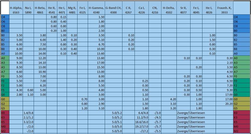
Determination of the spectral class according to Jaschek & Jaschek [1], problem
of luminosity class determination
In tables for the different spectral classes of main sequence stars, the authors give typical
equivalent widths for typical lines. For the purpose of overview, the data from [1] were
summarised in table 2.A good assignment to the searched for spectral class can be achieved by
analyzing several lines; this could be verified in numerous of my own measurements, also done in
low-resolution spectroscopy. Many of the described lines, especially the hydrogen lines, are well
resolved and easy to evaluate even in low-resolution spectra. The tolerance lies in the range of a
few angstroms and the spectral type can therefore vary from line to line.
BAV MAGAZINE SPECTROSCOPY 36BAV Magazine
SPEcTRoscopy
Photometry and Spectroscopy of Collinder 399
If the mean value is calculated from the assignment of several lines, the spectral class searched
for is very close. It should be noted that the data are only valid for stars of the main sequence.
Therefore, it is important to determine the luminosity class. In contrast to the temperature
determination, however, the assignment to the appropriate luminosity class is rather difficult.
Basically, the hydrogen lines are suitable for this determination; towards higher luminosity
classes they become narrower and sharper. This behaviour is called the negative luminosity
effect. This effect can be found in spectral classes A0 to A3. From A5 onwards the effect weakens
and is hardly perceptible from A7 onwards. In addition, other effects must be taken into account
that lead to a line broadening independent of the spectral class, such as the broadening due to
rotation in the case of rapidly rotating Be stars.
Tab. 2: Equivalent widths for prominent lines according to Jaschek & Jaschek
Since these effects cannot be detected in low-resolution spectra, a misinterpretation can
quickly occur and a Be giant is then wrongly classified as a B dwarf. A reliable determination of
the luminosity class is done by the calculation of the line ratio of metallic lines. Information on
this is found in the Bonner Spectral Atlas [6] and in the Spectral Atlas published by Gray/
Corbally [7].Unfortunately, most of the lines and line ratios listed here are not reliably
identifiable in the low-resolution spectra and thus cannot be used. Nevertheless, these two
standard works on spectral classification are worth consulting and using, as many valuable clues
BAV MAGAZINE SPECTROSCOPY 37BAV Magazine
SPEcTRoscopy
Photometry and Spectroscopy of Collinder 399
can be found here. In the end, the only way to estimate the LK class in this project was to
compare the equivalent widths of the hydrogen lines with the resulting uncertainty.
Determination of spectral class with my own "database”
Following the example of the table shown above in [1], a small database of 90 observations
was created from my own spectral images. These spectra range from Mintaka (O9 III) to
Betelgeuse M4 Ib, whereby some stars are represented several times by several observations.
Of course, it is advantageous that the measured equivalent widths were recorded with the
same setup that was used for Collinder 399. The multiple observations of individual stars also
reveal the range of errors in the measurements that slit-less spectroscopy, which is dependent on
seeing, has to deal with.
Although this does not ultimately lead to a clear determination of a spectral class, a possible
range can be narrowed down and thus provides a valuable contribution to the overall picture that
needs to be put together.
Determination of the spectral class with flow chart
In [2], a flow chart is used for a rough estimation of the spectral class, with which the
temperature component of the spectral class can be determined. Unfortunately, the assignment
of the luminosity class is not possible with this. It is also not possible to make a precise
determination of the spectral class, as the determined range often fluctuates over several
subclasses; in the project it was often the classes A0 to A5.
Estimation of the temperature with Planck curve
The flux calibration of my own spectra with a spectroscopic standard star (preferably of the
class A0V such as Vega) leads to a spectrum which is free of the instrument profile, and on which
a temperature estimation according to Wien's displacement law can be made on the basis of the
continuum shape.
For this purpose, a function is fitted to the continuum using the software Vspec [8] with the
help of the Auto Planck function, and the temperature is determined from this. The simple
method of flux calibration involves inaccuracies in its implementation, which result from
different atmospheric influences and the different interstellar extinction of the standard star and
the observed star. However, in the context of this project in low-resolution spectroscopy, the
achievable accuracy appears sufficient to make a rough temperature estimate.
BAV MAGAZINE SPECTROSCOPY 38BAV Magazine
SPEcTRoscopy
Photometry and Spectroscopy of Collinder 399
Fig. 6: 5 Vul in Vspec with fitted Planck curve of 11.300K
Summary of the spectral class determination
Table 3 shows the summary of the results obtained from the methods presented above and,
derived from this, the final determination of the spectral classes for the individual stars. The
derivation of the spectral class is explained using the example of 5 Vul. The equivalent
measurements of the hydrogen lines resulted in widths of 17 Å each for Hδ and Hγ and 15 Å for
Hß and Hα. According to Table 2, Hγ and Hß can be assigned very well to class A3, while Hα
deviates slightly and is more likely to be assigned to A0. In my own database also, the Hδ line is
measured, so that 4 line widths could be determined. Matching with this are stars like Vega (A0
V), Sirius (A1 V), Castor (A1 V) or Deneb (A3 V). Here we also find a clear indication of the
luminosity class; the stars with a higher luminosity class have significantly narrower widths in the
database. The flow chart does not allow any further specification of the spectral class and only
confirms the estimation already found.
The spectral class found by means of the Planck temperature curve is different; it is located
much earlier already at the end of the B class and therefore fits very well with the determined
range from the B-V colour index. Since the luminosity class was determined as a dwarf, the
classification can be made as B7 V at the earliest. Taking into account the measured EW widths
of the spectral lines, which suggest a later type, the classification is ultimately as B8-9 V. The
occurrence of atomic helium lines in the B class is understood as a distinction from the A class,
in which helium lines are no longer found. Even if no helium lines can be identified in the present
spectrum due to the low resolution, the assignment to the B-type appears justified due to the
small number of lines that can be evaluated. Although at higher resolution, for the range from
3900 to 4500 Å at A0, Gray/Corbally [7] give approximately 13 lines that can be evaluated,
while at F2 there are already 87. In the available spectrum of 5 Vul there are only 3 lines that can
be considered for evaluation in the mentioned line range. For all other stars, the spectral class
BAV MAGAZINE SPECTROSCOPY 39BAV Magazine
SPEcTRoscopy
Photometry and Spectroscopy of Collinder 399
stars have a significantly poorer signal-to-noise ratio and the assignment was often made with
remaining uncertainty.
Tab. 3: Overview of the spectral classes derived from the individual examination methods
Determination of absolute brightness and distance
The absolute magnitudes of the spectral classes determined can now be derived from a tabular
compilation by [2]. The author R. Walker refers to data from the University of Northern Iowa
on main sequence stars, and explicitly points out that the supplementary data on giants and
supergiants from his own sources do not show a clear trend in analogy to the main sequence
stars. Of the 50 spectral classes listed by him and completely documented with main sequence
stars, only 19 classes of giants and only 11 classes of supergiants are provided with corresponding
data. In the Collinder 399 project, 5 dwarfs, 1 subgiant and 3 giants were determined from the 9
evaluated spectra. The subgiant was assigned to the dwarfs; for the giants no information could
be found for HD 182422 (A0 III) and a rough estimate was made. For the other two giant stars,
corresponding magnitudes could be taken. With the help of the distance module already given
above, the measured apparent and determined absolute brightnesses could now be converted
into distances.
Tab. 4: Absolute brightness and distances as a dependency of the spectral class,
sorted in ascending order by distance
BAV MAGAZINE SPECTROSCOPY 40BAV Magazine
SPEcTRoscopy
Photometry and Spectroscopy of Collinder 399
Comparison of the determined spectral classes with literature values
The data on the spectral classes of the Simbad database [9] were included in Table 4 for
comparison. Taking into account that Simbad [9] also contains different information on the
spectral classes, the determination of the temperature portion of the MK classification appears to
be quite successful. In Simbad [9], for example, there are 8 specifications for the determination
of the spectral class for 5 Vulpecula with 5x A0V, 1x A0, 1x B9 V and 1x B9.
The assignment of the luminosity class results in 3 matches, 3 deviations from one luminosity
class and 3 deviations in the order of magnitude of 2 luminosity classes. This result also appears
to be quite acceptable on the first hand, taking into account the spectral quality and the lack of
higher resolution.
If one compares the determined distances with the literature data, one obtains 3 results with
deviations below 10%, 4 results with errors between 30 and 50%, 1 result with an error of
100% and 1 result with an error of 240%. If one now considers the errors of the spectral classes
determined by oneself with the literature, even minor deviations of 1-2 subclasses in
temperature result in errors of 30-40%.
On the other hand, misclassifications in temperature of 2-3 subclasses and the misclassification
dwarf/giant compensate each other and result in errors of about 50%. It becomes critical when
the misclassifications in temperature and luminosity class do not compensate each other, because
then the errors reach approximately 100% and even significantly more.
These large fluctuations are mainly due to the uncertainties in determining the absolute
brightness from the spectral class and here especially the luminosity class, as explained above. If,
for example, the absolute brightness of 5 Vulpecula is set to 1.5mag for the class A0 V, the value
of 72pc taken from the literature is obtained exactly.
Star cluster or asterism
Returning to the original question, it must be stated that even without knowledge of the
literature values and with the simultaneous assumption of a generous error consideration, the
differences in the distances between the stars are too great to represent an open star cluster with
stars of the same distance.
If, on the one hand, only the determined distances are taken into account without considering
errors, the differences in distance are so great that it can only be an asterism and not an open star
cluster. Although there is a group of 5 stars that are relatively equidistant by about 100pc and
would allow the conclusion that it could be a star cluster, there is a second group of 2 stars with a
distance of about 400pc and 2 stars with a distance of about 600pc, which by this difference in
BAV MAGAZINE SPECTROSCOPY 41You can also read