Big Bang, Big Data - J.-F. Cardoso, CNRS (Télécom-ParisTech, IAP, APC) with the the Planck collaboration École d'Été de Peyresq. Traitement du ...
←
→
Page content transcription
If your browser does not render page correctly, please read the page content below
Big Bang, Big Data

J.-F. Cardoso, CNRS (Télécom-ParisTech, IAP, APC) with the the Planck collaboration

École d’Été de Peyresq. Traitement du Signal et des Images. GRETSI et GdR ISIS. Juin 2014.
“The cosmos, back in the day”. Big Science, big news.
Notre plan

 1. La théorie (le Big Bang): un peu de cosmologie, l’histoire de l’Univers, à grands traits.

 2. Les observations: le satellite Planck; ce qu’il a vu, et comment.

 3. Leur recontre: extraire la Science des observations.
                                    L’âge de l’Univers est . . .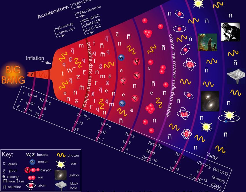
Préliminaire: des formes et des couleurs

La Terre mise à plat (projection de Mollweide) : un sphéroïde bleu, vert, jaune, blanc,. . . à l’oeil

Le rayonnement fossile, mesuré sur toute la voûte céleste, mis à plat.

Une carte de température en couleurs arbitraires.
.

    Big Bang

.
L’histoire de l’Univers en une image
Quand l’Univers devient transparent, la lumière se fossilise.
La plus vieille image du monde
Peut-on réellement percevoir une lumière si lointaine?

Deux gars l’ont vue, sans faire exprès, en 1965. Nobel pour Penzias et Wilson!

Et ils l’ont trouvée uniforme et froide: à peu près 3 degrés Kelvin. C’est-à-dire?

.
Lumière, matière et température
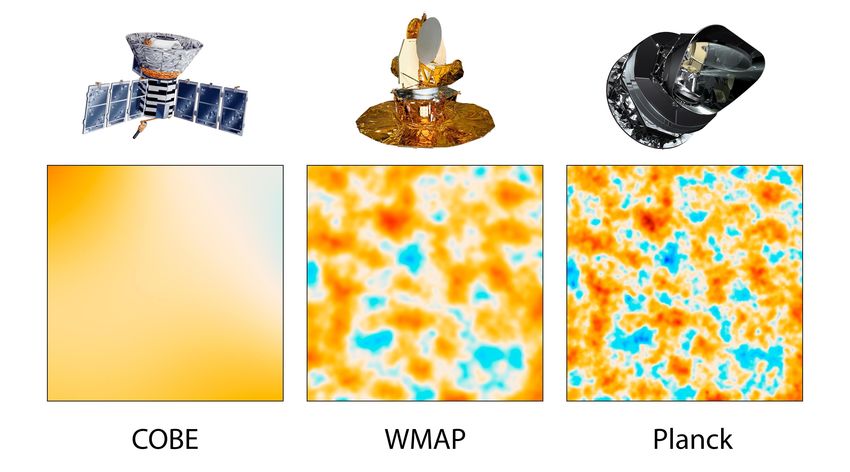
La théorie (Planck) Les mesures (COBE 1992)
La répartition d’énergie en function
de la fréquence ν d’un rayonnement
de température T est théorisée par la
loi de Planck
2hν 3 1
I(ν) = 2 hν/kT
c e −1
avec les honorables constantes:
• c: vitesse de la lumière
• h: constante de Planck
• k: constante de Boltzmann
Éblouissant accord entre la mesure et la forme théorique!
L’Univers est rempli de vieux photons froids à 2.725 degrés Kelvin.
Et donc, il s’est dilaté 1000 fois depuis la recombinaison: zrec ≈ 1000.Le rayonnement fossile est isotrope, mais pas trop Des anisotropies de 0,0001 degrés (Kelvin) et de 1 degré (centigrade).
L’Univers sauvé par les anisotropies

A peine âgé de 380,000 ans, l’Univers est dans une situation délicate:

                                                                                    .

Beaucoup reste donc à faire: les étoiles, les galaxies, les planètes, la vie. . .
Tout va-t-il donc partir à vau-l’eau? Il faut initier les grandes structures!
.
Planck
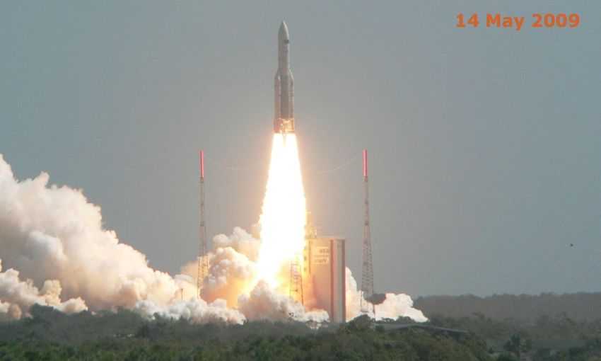
.Pour mieux y voir: la mission Planck
En route pour le deuxième point de Lagrange!!
Les cosmologistes adorent le 2ème point de Lagrange Terre-Soleil
Scanning the sky

Le téléscope focalise la lumière vers 52 cornets (HFI) qui la filtrent et la guident
vers les bolomètres refroidis à 0.1 degrés Kelvin.

Notez les tuyaux: Planck est aussi un exploit frigorifique.
Le plan focal de Planck HFI

                                   2
                                                                                   353-8   545-4

                                                                                353-7
                                                                                                         143-4
                                                                      217-8

                                   1
                                                     100-4
                                                              217-4                353-6     857-4

                    co-scan [◦ ]                                      217-7                              143-3
                                                              217-3             353-5       857-3
                                             100-3                                                               143-7
                                   0

                                                                                   353-4     857-2
                                                              217-2                                              143-6
                                             100-2
                                                                      217-6
                                                                                                         143-2
                                   −1

                                                                                353-3       857-1
                                                             217-1
                                                                      217-5                                      143-5
                                                     100-1
                                                                                   353-2   545-2         143-1
                                   −2

                                                                                353-1      545-1

                                        −2                   −1                0                     1              2
                                                                         cross-scan [◦ ]

5 arc-minute resolution in best channels → 50 106 pixels over the sky.
Les canaux spectraux moyens de Planck HFI
Wavenumber [cm-1]
5 10 20 30
1.0 0.8
Spectral Transmission
0.6
CO J=5→4
CO J=8→7
CO J=6→5
CO J=7→6
CO J=9→8
CO J=3→2
CO J=1→0
CO J=4→3
CO J=2→1
0.4
100 GHz
0.2
143 GHz
217 GHz
353 GHz
545 GHz
857 GHz
0.0
102 103
Frequency [GHz]Signals from a 143 GHz, a 545 GHz, a dark bolometer A serious case of glitchopathy.
Les mêmes, après deglitching

After some glitchotherapy (thanks to recent advances in glitchology).
Map Making needed

The cosmological signal is still under the noise.

How to go from noisy time lines to less noisy spherical maps:
another adventure in big data.
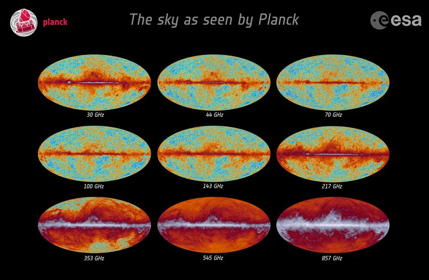
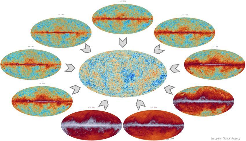
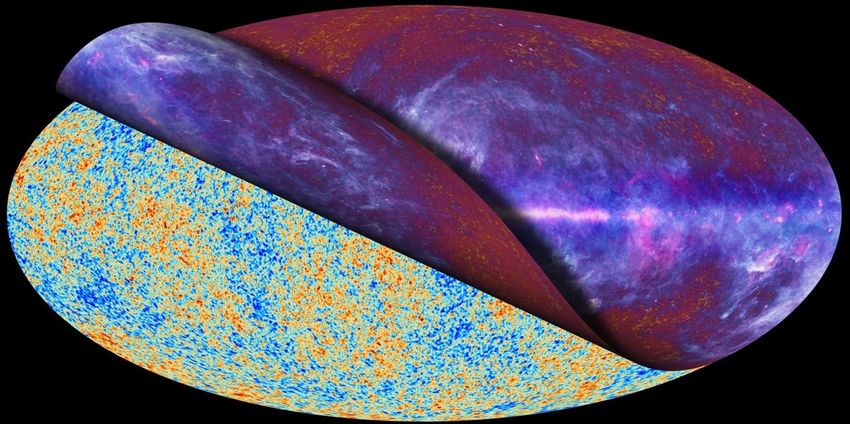
Combinaison des 9 canaux Planck pour extraire le rayonnement fossile
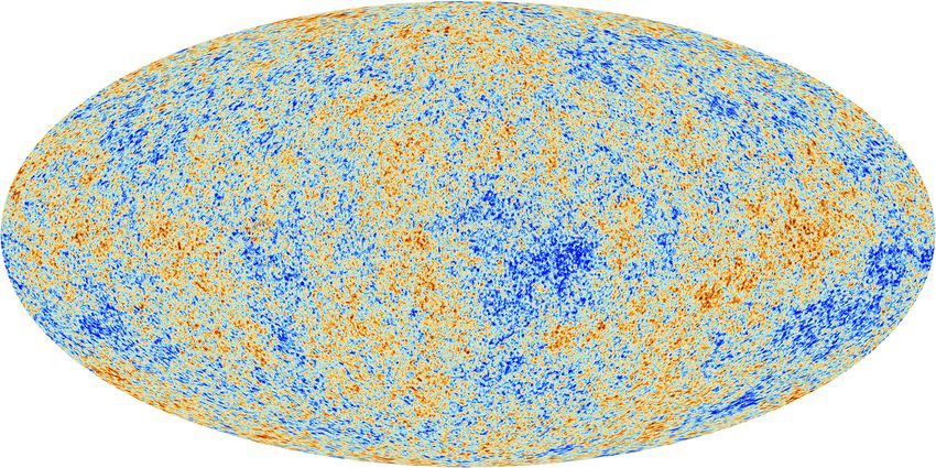
Credit: ESA, FRBLa plus vieille image du monde, par Planck
Echelle de couleur: ± 300 millionièmes de degré.COBE 1992, WMAP 2001, Planck 2013 Fine, but how does one do Science with such a boring image ?
.
Cosmological inference on the sphere
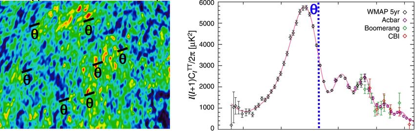
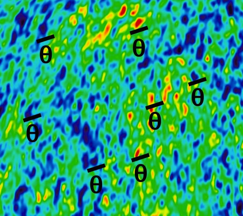
.Météo marine et analyse spectrale A gauche: Vent de nord-ouest, mer calme. A droite: Anisotropies de la température du rayonnement fossile: taille angulaire 1 degré, amplitude: 0,0001 degré Kelvin. Pourquoi nous voulons voir l’univers vibrer.
En route vers le quantitatif.

Toute l’information (ou presque) est contenue dans le spectre angulaire.

Il mesure la distribution de l’amplitude des fluctuations selon leur échelle.

La physique du plasma primordial se lit aux échelles plus fines que 1 degré.
So, we need to go spherical, don’t we ?

 • No universally satisfying pixelization.
   In particular, no easy translation by almost any amount.

 • Rotations and translations are the same thing.

 • The rotation group for the sphere SO(3) is not commutative.

 • There is no convolution on the sphere (although. . . )

 • There is no dilation without distortion (wavelets?).

 • We need a ‘good’ basis for the space of functions defined on the sphere.
   Here ‘good’ means: with the same symmetries as the sphere itself.

 • So, what is the Fourier basis?

 • And what is a “spherical frequency” in the first place?
Multipoles and angukar frequencies

A spherical field X(θ, φ) can decomposed into ‘harmonic’ components:
                     X (`)(θ, φ)
               X
   X(θ, φ) =                       [θ, φ] = [(co)latitude, longitude]
               `≥0
called monopole, dipole, quadrupole, octopole, . . . , multipole. Visually:

             =               +         +           +           +        + ···

Each multipole component can be characterized as the orthogonal projection
onto the `-th eigenspace of the spherical Laplacian ∆ = ∂ 2/∂x2 + ∂ 2/∂y 2:
   ∆X (`)(θ, φ) = −`(` + 1) X (`)(θ, φ)
Compare to the circular case: [∂ 2/∂θ2] eimθ = −m2 eimθ .

The `-th eigen-subspace of the spherical Laplacian,
• contains all functions at angular frequency (or multipole) `,
• is globally invariant under rotation,
• has dimension 2` + 1,
• has a nice orthonormal basis
Spherical harmonics
• An ortho-basis for spherical fields: the spherical harmonics Y`,m(θ, φ):
X m=−`
X Z Z
X(θ, φ) = a`,m Y`,m(θ, φ) ←→ a`,m = Y`,m(θ, φ) X(θ, φ)
`≥0 m=` θ φ
• Better than simply orthogonal: it factors as Y`,m(θ, φ) = eimφ P`,m(cos θ).
• So we have semi-fast spherical harmonic transforms. . .
. . . for good sampling schemes.
q
• Think of the double index (`, m) as a spherical version of kx2 + ky2, ky .
• The decomposition into multipoles:
m=−`
X (`)(θ, φ) =
X
a`,m Y`,m(θ, φ)
m=`Angular spectrum and likelihood
• The spherical harmonic coefficients a`,m of a stationary random field
are uncorrelated with variance C` called “the angular power spectrum” :
E a`,m a`0m0 = C` δ``0 δmm0 distribution of power vs angular frequency `.
• Thus, for a Gaussian field, the empirical spectrum
m=−`
1 2
a2
X
C` =
b Var C`/C` =
b (Cosmic variance)
2` + 1 m=` `,m 2` + 1
is a sufficient statistic, compressing all information since the likelihood reads:
C`
X b
−2 log P (X|{C`}) = (2` + 1) + log C` + cst Super compression!
`≥0
C`
• It is also a spectral mismatch:
X def
−2 log P (X|{C`}) = (2` + 1) k(Cb`/C`) + cst’ k(u) = u − log u − 1
`≥0Angular spectrum and likelihood
= + + + + + ···
X(θ, φ) = X (0)(θ, φ) + X (1)(θ, φ) + X (2)(θ, φ) + X (3)(θ, φ) + · · ·
def
The empirical angular spectrum Cb` = kX (`)k2/(2` + 1)
def
The “true” angular spectrum C` = E Cb`
We have only one sky, one observable Universe, one set of Cb`.
The “true” angular spectrum C` exists only in the theory.The likelihood of our Universe
• Cosmologists build physical models predicting a Gaussian stationary CMB sky
with an angular spectrum depending on fundamental cosmologic parameters:
C` = C`(α) α = (ΩΛ, Ωm, H0, . . .)
• Instrumentalists painfully measures the angular spectrum Cb` of the CMB sky.
• Statisticians know that Cb` then is a sufficient statistic: the likelihood reads:
!
X Cb`
−2 log p(CMB|α) = (2` + 1) + log C`(α) + cst.
`≥0
C`(α)
• In real life, things (the likelihood, the estimate Cb`) are much more complicated,
but we still match a model spectrum to an empirical spectrum.Theoretical angular spectrum of the CMB
A cosmological model has to
predict the angular spectrum of
the CMB as a function of “cos-
mological parameters”.
Left: examples of the depen-
dance of the spectrum on some
parameters of the Λ − CDM
model.
Important note : we plot `2C`.
Large scales dominate the power.W-MAP 5-year angular spectrum.
Plot of rescaled spectrum:
`(` + 1)
D(`) = C(`) ×
2π
Black ink: measures.
Red ink: best-fit theory spectrum.
Three acoustic peaks: congrats, W-MAP!
Note the puzzingly low quadrupole (harmonic frequency ` = 2)
Cosmic variance dominates for ` ≤ 540;
instrumental noise dominates at higher multipoles..
Component separation
.Extracting the CMB from the 9 Planck frequency channels Color scale: hundreds of micro-Kelvins. Credits: ESA, FRB.
Four CMB anisotropy maps delivered to the Planck Legacy Archive

        NILC             SEVEM                 SMICA             C-R
   `SNR=1 = 1790      `SNR=1 = 1790      `SNR=1 = 1790     `SNR=1 = 1550
    Wavelet space      Wawelet-like     Harmonic space       Pixel space
    non-parametric    non-parametric     semi-parametric      parametric

• Various assumptions about the foregrounds.

• Various filtering schemes (space-dependent, multipole-dependent, or both).

• The SMICA (Spectral Mismatch ICA) method selected for
the ‘Main product’ for the Planck CMB map.
Some requirements for producing a CMB map • The method should be accurate and high SNR (obviously). • The method should be linear in the data: 1. It is critical not to introduce non Gaussianity 2. Propagation of simulated individual inputs should be straightforward • The result should be easily described (e.g. map=beam*sky+noise) with a well defined transfer function. • The method should be fast enough for thousands of Monte-Carlo runs. • The method should be able to support wide dynamical ranges, over the sky, over angular frequencies, across channel frequencies.
Wide dynamics over the sky

Left: The W-MAP K band. Natural color scale [-200, 130000] µK.
Middle: Same map with an equalized color scale.
Right: Same map with a color scale adapted to CMB: [-300, 300] µK.

                                Average power as a function of latitude
                                on a log scale for the same map.

Do we really want to estimate covariance matrices over the whole sky?
Wide spectral dynamics, SNR variations C(`) b · `(` + 1)/2π in [µKRJ]2 for fsky = 0.99.
And what about the noise ?

Noise RMS in µK in the SMICA map.
Simple CMB cleaning by “template removal”

X143 GHz                    X353 GHz                    X143 GHz − αX
                                                                   b 353 GHz

Assume that the 353 GHz channel sees only dust emission
and that the 143 GHz channel sees CMB plus a rescaled dust pattern:
   X143 = CMB + α X353
                       b = hX143X353i/hX353X353i and a clean (?) CMB map as
Find α by correlation: α
                hX143X353i
   CMB = X143 −
    d                      X353        where h·i denotes a pixel average
                hX353X353i

The result (top right) does not look bad, but it is !

Note: By construction hCMB
                        d X
                            353 i = 0.
Combining all 9 Planck channels, non parametrically: the ILC
Stack the 9 Planck channels into a data 9 × 1 vector d = [d30, d44, . . . , d545, d857]†
and estimate the CMB signal s(p) in pixel p by weighting the inputs:
sb(p) = w†d(p) p = 1, . . . , Npix
At frequency ν, the CMB signal s(p) has amplitude aν and contaminated by fν (p)
dν (p) = aν s(p) + fν (p) or d(p) = a s(p) + f (p)
The best (minw h(s − w†d)2ip) unbiased (w†a = 1) estimator is:
b −1 a
C
w= b with Cb = hdd†i , the sample covariance matrix
p
† −1
a C a
That is known as ILC (Internal Linear Combination) in CMB circles, as MVBF
(Minimum Variance Beam Former) in array processing, otherwise elsewhere.
Looks good: linear, unbiased, minimum MSE, very blind, very few assumptions:
knowing a (calibration) and the CMB uncorrelated from the rest (very true).Is the ILC good enough for Planck data ?
A simulation result:
←− ILC map on a
±300µK color scale
Error on a ±50µK
color scale −→
ILC looked promising, but something went wrong.
Actually two things, at least, need fixing:
• harmonic dependence and
• chance correlations.SMICA: Linear filtering in harmonic space
Since resolution, noise and foregrounds vary (wildly) in power over channels and
angular frequency, the combining weights should depend on `.
The SMICA CMB map is synthesized
3
from spherical harmonic coefficients 217
2
ŝ`,m, obtained as linear combinations: 143
353
†
1
¤
ŝ`,m = w` d`,m with, again,
wi (`) µK/µKRJ
i
0
C−1
` a
£
w` = C` = Cov(d`,m) 100
a†C−1
` a
1
030 545
044
070 857
• At high `, the (spectral) covariance 100
143
2
217
matrices C` are well estimated by their 353
545
857
sample counterparts
3
500 1000 1500 2000 2500 3000 3500
• At lower `, we need to get smarter. `
Note: spectral localization is a must. Spatial localization do not seem critical (See NILC perf.).Foregrounds and how to get rid of them (at low `) ?
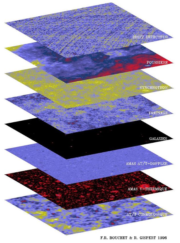
Various foreground emissions (both galactic and
extra-galactic) pile up in front of the CMB.
But they do so additively !
Noise
Even better, most scale rigidly with frequency: each
Dust
frequency channel sees a different mixture of each
Synchrotron astrophysical emission:
Free-free d = As + n (data = mixture x sources + noise)
Galaxies Such a linear mixture can be inverted . . . if the mixing
Gal clusters matrix A is known. How to find it or do without it ?
Gal clusters
1 Trust astrophysics and use parametric models, or
CMB
2 Trust your data and the power of statistics.Foregrounds, physical components and the mixing matrix
At low ` (i.e. large angular scales), there are less Fourier modes available for
estimating spectral statistics C
b : the variability (chance correlations) must be
`
decreased by fitting a model C`(θ) to Cb .
`
• Mixing matrix. The 9 Planck channels as noisy linear mixtures of components:
d`,m = A(θ) s`,m + n`,m
• Some models for the mixing matrix A = A(θ):
Type Mixing matrix parameters θ
physical, fixed A = [acmb adust aCO aLF] θ=[ ]
physical, parametric A = [acmb adust(T ) aCO aLF(β) ] θ = (T, β)
non-parametric (∼ ILC) A = [acmb B] (a square matrix) θ=B
semi-parametric, SMICA A = A (any tall matrix) θ=A
• Which model, which fitting criterion? See next the SMICA case.SMICA semi-parametric model
• SMICA models the 9 Planck channels as noisy linear mixtures of CMB and 6 “foregrounds”:
d1 a1 F11 . . . F16 n1
d2 a2 s
F21 . . . F26 n2
.. = ...
. ... f
... × 1 + ... or d
s`,m
... .
.. . `,m = [ a | F ] + n`,m
.
..
.
.. ... .
.. .. f `,m
...
f6
d9 a9 F91 . . . F96 n9
• SMICA only assumes decorrelation between foregrounds and CMB.
The foregrounds must have 6 (say) dimensions but are otherwise completely unconstrained:
they may have any spectrum, any color, any correlation. . .
So the data model is very blind: all non-zero parameters are free !
2
σ . . . 0
C`cmb 0 † .
.
1`
... ... = C (a, C cmb , F, P , σ 2 ).
Cov(d`,m ) = [ a | F ] [a | F] + . ` ` ` i`
0 P` 2
0 . . . σ9`
• Blind identifiability: can it be done? Maths say: yes!
−1
P
• Fit by minθ ` (2` + 1) trace C` C` (θ) + log det C` (θ) = Gaussian stationary likelihood.
b
• Only Span(A), the foreground subspace, is needed to suppress the foregrounds.
It is collectively determined by all the multipoles involved in the fit.Why the stationary Gaussian likelihood is OK (and sparsity useless)
" #
s
Consider the noise-free, square case : d = [ a | F ] with known a.
f
For any matrix G, the ‘preprocessor’ T = [ a | G ]−1 ensures
1 α† s + α† f
" # " #
TA = [ a | G ]−1 [ a | F ] = so that d
e = Td =
0 Y Yf
Hence, the first pre-processed channel d
e contains the signal of interest s
1
contaminated by a linear combination of the other observed channels d e , de ,···.
2 3
• Statistical foreground models not needed: they are deterministically observed.
• Hence, a statistical model is needed only for the CMB. Since it is Gaussian and
stationary, the likelihood has a simple expression which is readily maximized in the
cleaning coefficients. That justifies the use of a Gaussian stationary likelihood
for fitting the SMICA model.More explicitly
Assuming without loss of generality that Y = Id and denoting d = d̃1, the model
is, in each pixel p
d(p) = s(p) + α† f (p)
with f (p) observed. For the best cleaning, we need the optimal estimate of α.
But the likelihood is trivial in harmonic space, with the CMB as ‘noise’ (!)
X (d`,m − α†f`,m)2
−2 log P (d|α) = (2` + 1) + cst
`
C`
The (trivial) solution corresponds to combining the inputs with weight vector
b −1 a
C
d`,md†`,m/C`
XX
w= b i.e. an ILC with C
b =
a†C−1 a ` m
This is also the SMICA solution in the same context:
chance correlation is optimally mitigated in the spectral domain..
Results
.The big pipeline picture, from time series to cosmology, ideally
← SCANNING THE SKY.
Make sure you capture those µKs in your time lines.
Deglitch, flag, deconvolve, calibrate. . .
← MAP MAKING: from time lines to spherical maps.
Here, the microwave sky at 23 GHz seen by W-MAP.
← COMPONENT SEPARATION: from several frequency channels maps
to a component map. Here, pure (?) CMB from WMAP.
← SPECTRAL ESTIMATION: a bumpy ‘angular spectrum’.
← LIKELIHOOD ANALYSIS. Here, likelihood of matter Ωm and vacuum Ω
energy densities in front of CMB data (and supernovae).
→ “Thus”, the Universe is flat and 13.7 ± 0.2 billions years old (says WMAP). . .Spectre angulaire de la carte Planck sur 89% du ciel. Sept pics acoustiques, woohoo! Les erreurs sont dominées par la variance cosmique jusqu’à ` = 1500 (disons).
Le spectre angulaire de Planck: contact entre théorie et observations

Un superbe ajustement des mesures par les prédictions du plus simple des modèles
cosmologiques: le modèle Λ − CDM à 6 paramètres.
Le modèle standard du Big Bang

Un scénario à 6 paramètres: Le modèle Λ-CDM.

    1.   Amplitude A des fluctuations primordiales
    2.   Leur indice spectral ns
    3.   Densité de matière noire Ωd
    4.   Densité d’énergie noire ΩΛ
    5.   Taux d’expansion Ho de l’Univers
    6.   Profondeur optique de ré-ionisation τ

.

Les 2 premiers paramètres A et ns décrivent le spectre primordial → inflation.

Les trois suivants Ho, Ωd, ΩΛ contrôlent sa “mise en forme”.
Quelques résultats Un taux d’expansion Ho de 67,15 km/s/Mpc et un âge de 13,8 milliards d’années.
Planck results

 • La plus grosse surprise: pas de grosse surprise.

 • Excellente prédiction des observations avec un modèle simple. . .
   mais un peu bizarre: Λ-CDM = inconnu + inconnu !

 • Sans parler de quelques anomalies marginales. . .

 • Beaucoup d’autres façons d’exploter les données Planck,
   tant en Cosmologie qu’en Astrophysique.

 • Magnifique succès scientifique, mais ce n’est pas fini. . .
Plus de science: lentillage gravitationnel

A movie
Plus de science: lentillage gravitationnel

A movie
Big Data ? Who has the biggest?
For HFI: 52 bolometers (2 broken) plus 2 ”darks” (plus 16 ancillary channels: thermometers,. . . )

Mission lasts as long as Helium: our fridge achieved > 2.5 years = 5 sky (about 1000 days).

1000 days of 24 hours of 60 minutes of 60 secs of 180 samples from 52 bolometers ∼ 8·1011 bytes.

• Compression with various kinds of redundancy:
From timelines to rings: a factor of ≈ 40
From rings to spherical maps: about 5000 rings per sky, maps of 12 · 20482 ∼ 50 · 106 pixels
From detector maps to frequency channel maps (several bolometers for a frequency band)
From 9 frequency channel maps to one CMB map
From one map to a angular spectrum: all multipoles have SNR > 1 up to ` ≈ 1800
From the angular spectrum to 6 cosmological parameters
→ Ultimate data size: 6 bytes.

• Bad/sad reasons for dumping data:
Instability after depointing: 1 minute per ring
Bad compression tuning in front of bright sources (was quickly fixed)
Dump data if dark bolos appear inconsistent (for whatever reason)
Nasty comsic rays give nasty glitches.
→ In the end 30% of the scientific data had to be discarded.
Thanks and get ready for polarization!
You can also read