Bitcoin High-Frequency Trend Prediction with Convolutional and Recurrent Neural Networks
←
→
Page content transcription
If your browser does not render page correctly, please read the page content below
Bitcoin High-Frequency Trend Prediction
     with Convolutional and Recurrent Neural
                    Networks
                                       Zihan Qiang                                 Jingyu Shen
                                     Stanford University                        Stanford University
                                    zqiang@stanford.edu                     jingyu.shen@stanford.edu

                                                             March 17, 2021
                                                                   Abstract

    Cryptocurrencies, with Bitcoins created in 2009 as the forerunner, can be exchanged, with the state-of-the-art block-chain technology
    providing protections for transactions. In this work, the deep learning techniques of convolutional neural networks (CNN) and long
    short-term memory (LSTM) networks are used as classification algorithms to perform one-step ahead high-frequency trend predictions
    of Bitcoin prices using minute level technical indicators. A hybrid CNN-LSTM model has been developed after many rounds of
    hyperparameter tuning. Our work has shown promising results that the developed model can, to a certain degree, extract useful signals
    from technical indicators and generate trading strategies that outperform the benchmark strategy of passively holding Bitcoins in terms
    of net asset value and Sharpe ratio in the backtesting period. A future plan of applying rolling window cross validation is also proposed.

                     I.   Introduction                                      cantly outperform others. In another research, by using 18
                                                                            technical indicators calculated from minute-level Bitcoin
In recent years, cryptocurrencies, especially Bitcoins, have                prices, Alonso-Monsalve, Suarez-Cetrulo, Cervantes, &
been gathering widespread public interest since its price                   Quintana, have used CNN, hybrid CNN-LSTM network,
spike in 2017 to $19,783 USD and a recent surge to around                   MLP, and RBF neural network to predict the price changes
$40,000 USD in January 2021. Due to the extremely volatile                  of the six most popular cryptocurrencies - Bitcoin, Dash,
and manipulation-prone nature, there have been ongoing                      Ether, Litecoin, Monero and Ripple, and have concluded
controversies around whether the cryptocurrency mar-                        that the hybrid CNN-LSTM network performs the best,
ket is a good place for investment. In this project, we                     with test accuracies reaching as high as 80% and 74% in
aim to forecast the minute level price changes of Bitcoins                  predicting price changes of Monero and Dash respectively.
traded on Binance using convolutional and recurrent neu-                    Bergmeir & Benítez, has tested the method of blocked
ral networks to generate investment strategies that can                     cross-validation on one-step ahead time series forecasting,
outperform the traditional strategy of passively holding                    which we call rolling windows cross-validation in this re-
assets. The inputs to our algorithms are the minute level                   port, to make use of the most recent information for each
open, close, high, and low prices, all represented as ex-                   round of validation process, and has yielded robust error
change rates with $USD, as well as the volume traded at                     estimates. We plan to re-calibrate and improve the CNN
Binance Bitcoin exchange and the overall volume traded in                   and CNN-LSTM hybrid model by using additional fea-
the market. Our algorithm will then predict the direction                   tures and including the most recent roller-coaster Bitcoin
of Bitcoin price change the next minute using the trained                   price fluctuations, which may provide more meaningful
algorithms.                                                                 implications going forward.

               II.    Literature Review                                                  III.    Dataset and Features
Deep learning algorithms have been applied and tested                       The dollar-denominated minute level Bitcoin prices and
in various research, some of which have shown accurate                      volumes from July 8, 2020 to Feb 11, 2021 are collected
yet robust results in Bitcoin’s high-frequency trend predic-                with a total of 313,327 data points, and 313,327 labels
tion. Ji, Kim, & Im, have tried deep learning algorithms                    of price change are generated, where 0 and 1 denote a
of DNN, LSTM, CNN, and RNN to predict Bitcoin re-                           decrease and an increase in price respectively. The entire
turns. The accuracy of these methods is around 50% to                       dataset is split into three parts, where the first 80% of the
60% and it is concluded that no methods would signifi-                      data are used as the training set, and the rest are equally

                                                                        1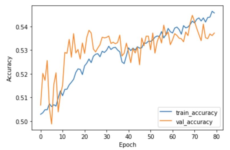
Bitcoin High-Frequency Trend Prediction with Convolutional and Recurrent Neural Networks

divided into dev and test sets. The following table shows                         are used to normalize the indicators in the validation and
the summary and balance of each dataset with respect to                           test sets.
the labels.

                      Labels     Samples         Percentages                                            IV.    Methods
           Train        0        125,444           49.18%
                        1        129,621           50.82%                         The model implemented in this paper includes two major
           Dev          0         14,330           50.55%                         components: CNN and LSTM.
                        1         14,017           49.45%
           Test         0         14,899           49.77%
                        1         15,016           50.23%                         i.   Convolutional Neural Networks
                      Table 1: Dataset Summary                                    The architecture of convolutional neural networks (CNN)
                                                                                  is used in our project to utilize its ability to exploit relation-
  Table 1 has shown that the labelling classes of three                           ships among adjacent data and to speed up the processing
datasets are well balanced, with both labels occupying 50%                        of the massive amount of high frequency data.
in each set, and do not have class imbalance issues. The                             To implement CNN, our minute level data points are
inputs are then used to calculate 30 technical indicators,                        first converted to a set of 2 dimensional "images" shaded
similar to the ones in Alonso-Monsalve et al., with some                          in blue as shown in Figure 1, with the 2 dimensions being
additions, as shown in Table 2.                                                   time lags (height) and technical indicators (width). Every
                                                                                  input image covers all of the 30 indicators and a certain
      Indicator                              Formula                              number of time lags for a given time stamp in our data.
     MOM(n, t)                               Ct − Ct−n                            The number of technical indicators are fixed throughout
                                                                                  the project whereas the number of time lags are fine tuned
     MOMret (n, t)                           log( CCt−t n )
                                                                                  as hyperparameters (the number of lags is shown as 15 in
                                      ∑in=−01 log(Ct−i /Ct−i−1 )
      SMAret (n, t)                                 n                             Figure 1 and 2 for the purpose of illustration). The direc-
                                 ∑in=−01 (n−i )×log(Ct−i /Ct−i−1 )                tion of the next minute price change, shaded in orange, is
     W MAret (n, t)                                 n
                                                                                  used as the label of a specific input "image".
       RSI (n, t)                       100 − ( 100       nup )
                                                     1+ n
                                                          down
                                                Ct − Lown
        SK (n, t)                          ( High  n − Lown
                                                             )
                                          10−1
       SD10 (n, t)                    ∑i=0 SK (n, t − i )
                                               Highn −Ct
       LWR(n, t)                           ( High  n − Lown
                                                             )
                              1/3×( Highn + Lown +Ct )−SMA(n,t)
      CCI (n, t)                           0.015× MD (n,t)
      MACD (t)              EW MA12                              26
                                        close ( t ) − EW MAclose ( t )
    ADOSCBinance (t)               3           (t) − EW MA10
                           EW MAV
                                      Binance                    VBinance ( t )
     ADOSCall (t)            EW MA3V (t) − EW MA10               Vall ( t )
                                           all

n ∈ {5, 10, 30}; Ct : close price at time t; nup , ndown : averages of
 n-day up and down closes; Highn , Lown : highest and lowest
price from last n periods; The subscript of EWMA denotes data
                                                                                               Figure 1: Two Examples of Data Points
        and the superscript denotes the lookback period.

                      Table 2: Technical Indicators                                 During the construction of our convolutional neural
                                                                                  network algorithm, we choose to use 1-dimensional filters
   The indicators of simple moving average and weighted                           that encode information of time series of a given indicator
moving average in the original paper are changed to be                            (vertical filters) or of a set of indicators at a given time
SMA and WMA of Bitcoin returns to ensure stationarity.                            (horizontal filters) as in Figure 2. The filter sizes are also
The calculation of technical indicators can be viewed as                          tuned as hyperparameters throughout the course of the
a transfer learning process that extracts useful features                         project. 1-D filters are been applied instead of 2-D filters,
of price dynamics, including momentum, relationships                              which are widely used in computer vision, because as a
among recent price levels, overbought and oversold condi-                         2-D filter slides through our input "images", the nature of
tions, and the overall accumulation and distribution. All                         the information that a given filter encodes is constantly
the above indicators in the training set are normalized,                          changing for each iteration (i.e. the filter looks at different
and the corresponding parameters of mean and variance                             indicators at different time stamps).

2
Bitcoin High-Frequency Trend Prediction with Convolutional and Recurrent Neural Networks
architecture, and will take the output of the CNN layers
as inputs. The optimal architecture of our LSTM network
is illustrated in Figure 4.
Our LSTM architecture consists of a 2-layer deep ver-
sion of LSTM. The output units of each layer is 100. It
means that the input 28 timestep by 10 features matrix
Figure 2: 1-D Filters will been fed into this model and transformed into 28 1 by
100 vectors first and eventually into one 1 by 100 vector.
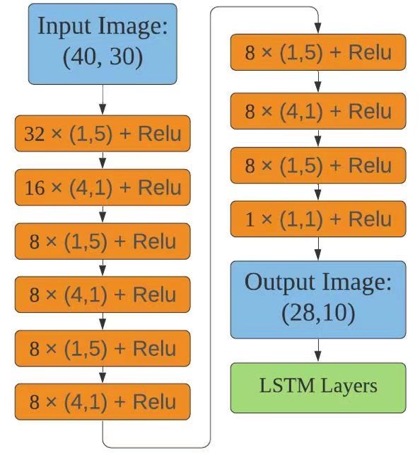
After tuning hyperparameters, we achieved the optimal This layer is then followed by a dense layer to generate
structure of our CNN model shown below in Figure 3. the label output with sigmoid activation function, which
Batch normalization layers are used in each convolutoinal takes on the value of 0 or 1. Dropout factors are added
layer to speed up training. Pooling layers are not used in the recurrent layers as well as in the dense layer as
in our CNN architecture because our input ’images’ are regularization to our architecture.
relatively small compared to the more commonly seen
RGB images which often have significantly larger sizes,
and the use of pooling layers can summarize the features
too early.
Figure 4: LSTM Layers
iii. Temporal Cross Validation
As our project is dealing with a time series data of Bit-
Figure 3: CNN Layers coins that do not have a well-defined nature, unlike other
popular asset classes such as stocks, bonds, and futures
The optimal lag for the input ’images’ is 40, and so the whose values are based on the corresponding companies,
CNN layers take the input of size 40 by 30 and return the governments, and the underlying assets respectively, the
output of size 28 by 10 after going through the filters. The distribution of Bitcoin’s historical data are constantly ex-
output ’images’ are inputted into the LSTM networks as periencing imperceptible shifts. Therefore, the methods
described in Section ii. of temporal cross validation is a preferable choice to vali-
date our models by keeping up-to-date with the market
ii. Long Short-Term Memory Networks conditions.
One method of rolling windows cross validation is
The long short-term memory (LSTM) networks are used in shown in Figure 5 below. For this method, there are a
our project to further exploit the sequential relationships number of rolling windows (5 in the figure for illustra-
among Bitcoin data, which, in our case, are time series tion), with each consisting of a training and validation set
data of technical indicators. It is an ideal tool for time- and the size of each set is kept the same for each rolling
series forecasting given its capability of dealing with the window. In each window, a training-validation process is
entire sequence of data. The two deep LSTM layers are performed, after which the window is moved in time by
added as additional layers to our already established CNN the amount of data points in the validation set, so that the
3Bitcoin High-Frequency Trend Prediction with Convolutional and Recurrent Neural Networks
next training set gets updated by adding the previous val- unchanged in the tuning process, as one of the literature
idation set and discarding the data points that are further implemented similar size and number of filters and have
in the past. achieved reasonable results. We make the vertical filter
size smaller than horizontal filter so the LSTM can capture
more time-series signals. The most important hyperpa-
rameters we tuned is the number of layers, where we tried
the number of layers all the way from 4 to 10 and ended
up with 5 horizontal and 4 vertical layers. The reason
why we have one less vertical filter is that, again, we pre-
fer to use LSTM, instead of CNN, to capture time-series
relationship.
The hyperparamters to tune in the LSTM layers are the
output units and number of LSTM layers. We mainly
tuned the output units of LSTM, all the way from 30 to
Figure 5: Rolling Windows Cross Validation 150 units, and choose to fix the LSTM layers to 2 as the
LSTM layers are typically no more than 3. We ended up
with 100 units to increase the model complexity while
However, the mentioned validation method has high keeping the algorithm computationally feasible.
computational cost and is not feasible for the scope of this The hyperparameters tuned in the overall hybrid model
project. Instead, we choose to select K independent blocks are batch size, epochs and dropout rate. We chose the
of data, as shown in Figure 6 below, and break them down batch size from 64 to 256 and the epochs from 80 to 120 for
into training and validation sets to evaluate the algorithm’s different cases to ensure convergence while save training
performance throughout different historical periods. The time. We tried dropout factors of 0.2 to 0.4 to add regular-
data used in the training-validation can shrink for large ization effect, and ended up with 0.2 dropout rate as 0.3
K’s, which may solve the distributional shift. For the and 0.4 would result in non-converging training loss.
evaluation of both methods, we use the average of our
algorithm’s performances on each validation sets.
VI. Results & Discussion
We trained the aforementioned model with Adam as the
optimizer, the binary cross-entropy function as the loss
function, and hyperparameters mentioned before. As sug-
gested in the section Temporal Cross Validation, we have
trained the model on K = 1,2,3 for testing purposes. As
this project is intended to generate optimal Bitcoin trading
strategies for investors by capturing signals from historical
data, the metrics of net asset value (NAV) and Sharpe ratio
Figure 6: Independent Cross Validation (SR), which are commonly used in the financial industry,
are used in addition to predictive accuracy. NAV mea-
sures the value of an investor’s asset at the end of the
V. Experiments investment horizon assuming 1 dollar is invested at the
beginning. The results for K = 1 are shown below. Note
The hyperparameters of the aforementioned model have that for each case, we trained for 3 times and average the
been fine tuned in great efforts. Note that the hyperpa- results to ensure robustness.
rameters of CNN layers are tuned together with the LSTM
layers. We start off the tuning process by trying to overfit Valid BTC NAV NAV BTC SR SR Acc
the training set, and then add dropout and regularization K=1 1.194 1.613 0.003 0.0078 0.514
to achieve the balance between bias and variance. Test BTC NAV NAV BTC SR SR Acc
In our CNN architecture, we experimented the hyperpa- K=1 1.29 1.455 0.0052 0.0074 0.511
rameters that affect the complexity of our model - number
of layers, number and size of filters at each layer. The train- Table 3: K = 1 Validation and Test Set Results
ing loss did not decrease dramatically in the beginning,
and thus we need to tune the above hyperparameters to We can observe that the valid and test accuracy are just
increase the model complexity in order to capture more above the 50% threshold, meaning that our model is not
signals. The number and size of filters remain relatively confident at predicting the next minute return. It is likely
4Bitcoin High-Frequency Trend Prediction with Convolutional and Recurrent Neural Networks
to be caused by a large distributional shift between our 34% return while Bitcoin has increased 23%. The profit
training set and validation or test test. The fundamentals from K = 2 is not as good as K = 1 as we are training on
have changed over the period so that the signal we learnt less data which may results in less signals being captured,
from training set is not effective in validation set. However, however, it is more robust given the higher accuracy with
we can see that the NAV and Sharpe ratio generated by less distributional shift.
our model outperforms the passive strategy. Our model For K = 3, we have observed that the accuracy is 0.507
can utilize past signal to generate trading strategies that and the validation loss is even increasing. It means that the
can outperform the benchmark. we have learnt noises or overfitted given that the training
We then tested with the temporal cross validation. The set is too short. Moreover, the NAV and Sharpe Ratio
results for K = 2 and K = 3 are shown below. Note that have underperformed the passive investing strategy. It
the results are the average over 2 or 3 trials. can be caused by the ineffective trained strategy, and the
validation set may also be too short to realize the strategy.
BTC NAV NAV BTC SR SR Acc In general, we have observed the distributional shift
K=2 1.23 1.34 0.013 0.018 0.53 when K = 1. Then, we tried to reduce the training set
K=3 1.10 1.02 0.0082 0.0008 0.507 by splitting the current dataset into 2 and 3 independent
blocks (K = 2,3). We realized that K = 2 would be a good
Table 4: K = 2 and 3 Validation results balance between the demand of short training set to offset
distributional shift and the demand of long training set to
We can observe that the accuracy when K = 2 is around offset overfitting. As suggested in section 4.3, we should
53%, which is much higher than K = 1. When K = 2, both further test the K = 2 strategy (i.e. the same length of
the training and validation set have been shortened, which training and validation) on the rolling basis to test out the
clearly offsets the distributional shift issue. It demon- stability of this strategy.
strates that the model is relatively good at predicting the
next minute return. Moreover, the NAV and Sharpe ratio
have outperformed the passive investing strategy. The VII. Conclusion
accuracy and NAV of one trial have been plotted below.
In this paper, we have implemented a hybrid deep learn-
ing model that includes CNN and LSTM to predict the
Bitcoin returns and generate investment strategy. 30 tech-
nical indicators have been computed as the features. We
then generated the input images by cropping the dataset
with time lag = 40. Next, we designed a CNN model
that is comprised of 9 layers with 5 horizontal filters to
encode relationships among features and 4 vertical layers
to encode those among time steps. Then, the output image
is fed into a 2 layer LSTM model with 100 units to further
capture the time-series. Finally, a sigmoid dense layer
Figure 7: K = 2 Accuracy is added to produce the binary result. Overall, the batch
normalization and dropout layers are also added to ensure
the regularization effect to avoid the overfitting. We first
trained the entire dataset and get only 51% accuracy but a
good NAV and Sharpe ratio, which outperforms passive
investing in Bitcoin. Although it suggests that there is
a distributional shift between train and validation which
causes lower accuracy, signals from the past are captures
to generate an outperforming investment strategy. We
then implemented the temporal cross validation (split),
and achieved 53% accuracy with better NAV and Sharpe
ratio when K = 2. We realized that the shortened training
set resolves the distributional shift issue, but is also suffi-
cient to capture the signals from historical data. For K =
3, the accuracy and NAV is too low as the model learns
Figure 8: K = 2 Net Asset Value only the noise. The next step would be to implement a
rolling temporal CV with the same length of training and
From Table 4, we can see that our strategy generated validation data as K = 2 to further test the strategy.
5Bitcoin High-Frequency Trend Prediction with Convolutional and Recurrent Neural Networks
VIII. Contributions iii. Accuracy and NAV for K = 3
Zihan Qiang and Jingyu Shen constantly and closely col-
laborated with each other. There is no clear line that could
separate the work. In general, they contributed equally to
this work.
IX. Appendix
i. Accuracy for K = 1
Figure 12: K = 3 Accuracy
Figure 9: K = 1 Valid Accuracy
ii. NAV for K = 1 Figure 13: K = 3 NAV
References
Alonso-Monsalve, S., Suarez-Cetrulo, A. L., Cervantes, A.,
Quintana, D. (2020). Convolution on neural net-
works for high-frequency trend prediction of cryp-
tocurrency exchange rates using technical indicators.
Expert Systems with Applications, 149, 113250.
Bergmeir, C., Benítez, J. M. (2012). On the
use of cross-validation for time series predictor
evaluation. Information Sciences, 191, 192-213.
Retrieved from https://www.sciencedirect.com/
Figure 10: K = 1 Valid NAV science/article/pii/S0020025511006773 (Data
Mining for Software Trustworthiness) doi: https://
doi.org/10.1016/j.ins.2011.12.028
Ji, S., Kim, J., Im, H. (2019). A comparative study of bitcoin
price prediction using deep learning. Mathematics,
7(10), 898.
Figure 11: K = 1 Test NAV
6You can also read